Energy-Positive House: Performance Assessment through Simulation and Measurement

Abstract

This paper presents the results for the operating energy performance of the smart operation for a low carbon energy region (SOLCER) house. The house design is based on a ‘systems’ approach, which integrates the building technologies for electrical and thermal energy systems, together with the architectural design. It is based on the concept of ‘energy positive’ buildings, utilising renewable energy systems which form part of the building envelope construction. The paper describes how the building energy model HTB2, with a range of additional ‘plugins’, has been used to simulate specific elements of the design and the overall energy performance of the house. Measurement data have been used in combination with the energy simulation results to evaluate the performance of the building together with its systems, and identifying the energy performance of individual components of the building. The study has indicated that an energy-positive performance can be achieved through an integrative systems approach. The analysis has indicated that the house, under normal occupancy, needs to import about 26% of its energy from the grid, but over the year its potential export to import ratio can reach 1.3:1. The paper discusses the performance gap between design and operation. It also considers the contribution of a transpired solar air collector (TSC) to space heating. The results have been used to gain a detailed understanding of energy-positive performance.

1. Introduction

To meet the target of a 100% reduction in the UK’s carbon emissions by 2050 [1], it is necessary to reduce the carbon emissions associated with the residential sector, which accounts for some 17% of the UK’s total energy consumption in 2017 [2]. The UK has set a target of nearly-zero-energy new housing in compliance with the EU directive [3], by the end of 2020, which means ‘a building that has a very high energy performance’, where the ‘nearly zero or very low amount of energy required should be covered to a very significant extent by energy from renewable sources, including energy from renewable sources produced on-site or nearby’. The regulated energy in the UK is for heating, cooling, lighting and ventilation. Under the forthcoming regulation changes, renewable energy will also potentially contribute to the unregulated electrical appliance loads. Even so, in most cases there will still be a net energy import from the grid over the whole year [4,5].

A zero-energy building (ZEB) can be defined as a net zero emission building in terms of carbon dioxide emissions, where the carbon emissions generated from grid-based fossil fuel energy use are balanced by the renewable energy generation on the building itself [6]. Case studies in a number of countries have shown the potential for zero-energy housing [7,8]. They are usually grid connected, and the zero-energy performance is based on the annual net zero input and output from the grid. There are also examples of off-grid zero-energy autonomous housing [9], although this would be more challenging. Total autonomy is not necessary unless the building is off-grid: the combination of renewable energy supply and energy storage to provide total autonomy will generally be too expensive and impractical in relation to the size of systems needed. In most situations the grid is available, so it can be used. In future the grid itself will become increasingly decarbonised with a higher proportion of large-scale renewable energy generation connected to it, for example, from wind farms and large-scale solar [10].

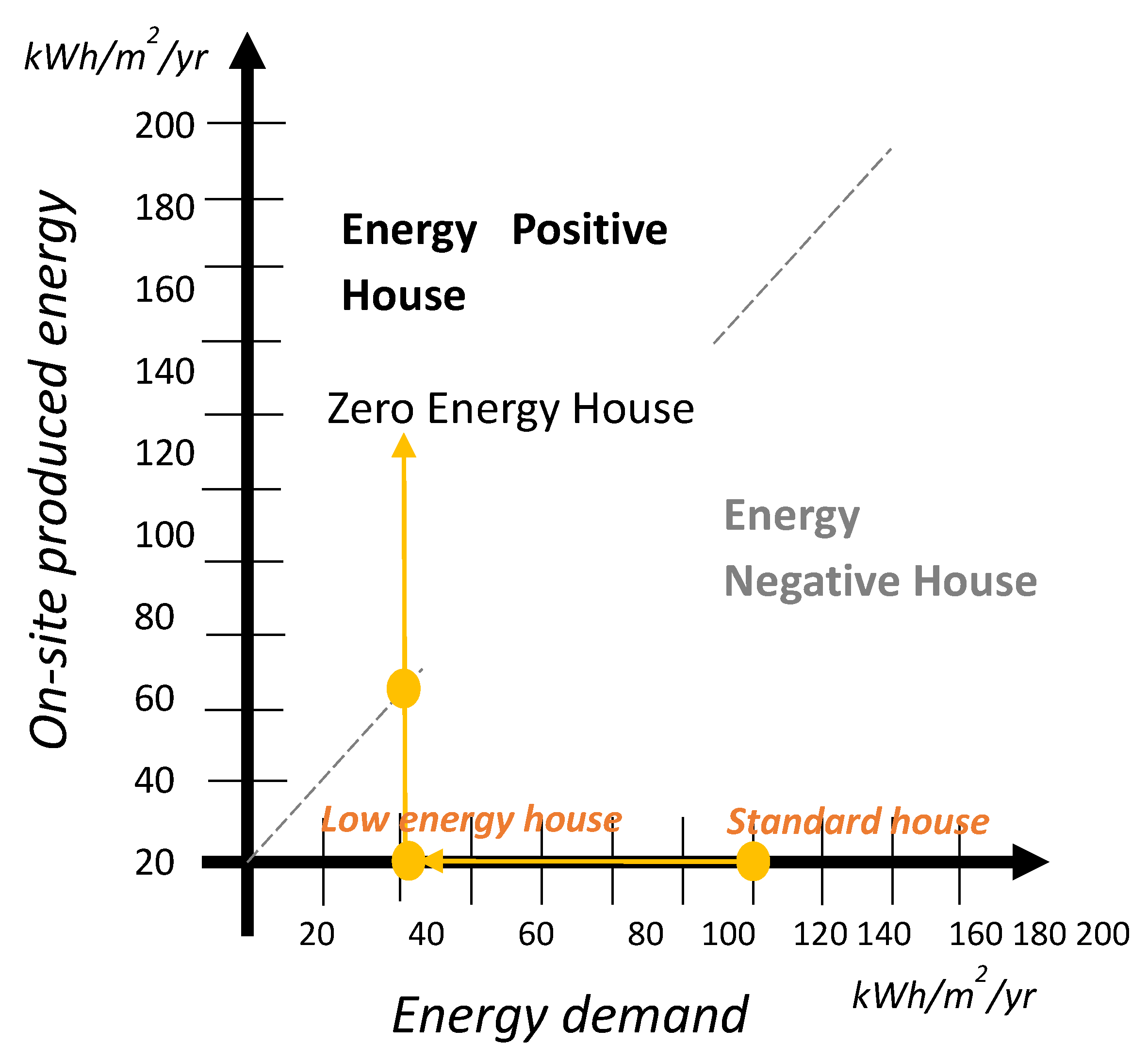
An energy-positive building can be defined, as a building where the total energy generated over the year is significantly greater than the energy needed to operate the building, including heating, ventilation, lighting and appliances [11]. Energy-positive buildings are generally based on a Passivhaus approach to reduce demand [12,13], with renewable energy generation a major feature [14]. An early example is the Frieburg Solar Community [15], which demonstrated that a whole estate could achieve energy-positive performance, although some individual houses could not due to design variations. Figure 1 illustrates the energy-positive performance in relation to energy demand and renewable supply.

A whole-house system approach integrates across passive design, efficient heating and ventilation, and the use of renewables [17,18]. The use of heat pumps is generally applicable for energy-positive housing, where a lower-temperature heating system is more appropriate [19]. Research has identified the importance of the balance between renewable energy and heat pump performance and opportunities for heat recovery in colder climates [20,21]. Simulation has been used to show the potential of energy-positive performance for groups of houses using heat pump technology [22].

There is currently a shift in European housing, from gas to electric heating, with the smart integration of solar PV (photovoltaic), heat pump technology and energy storage [23]. The UK Committee on Climate Change report, UK housing: Fit for the future [24] has recommended that from 2025 at the latest, no new homes should be connected to the gas grid. They should instead be heated through low carbon sources, have ultra-high levels of energy efficiency, alongside appropriate ventilation and, where possible, be timber-framed. It also recognises that addressing the ‘performance gap’ in new homes could save between £70 and £260 in energy bills per household per year.

Energy storage may be used to maximise the self-consumption of renewable energy used in the building [25,26], including heating domestic hot water [27]. Energy storage may be based on electricity, for example battery storage, or on thermal energy, for example energy stored in hot water, or in the construction materials of the building. Energy storage does not directly save energy, but it does reduce the amount of energy imported from the grid, which may contribute to reducing peak loads, and therefore ‘destressing’ the grid. From a householder’s point of view, in the UK, importing electricity from the grid incurs a higher cost compared to any payment received from exporting renewable energy to the grid. So from a householder’s point of view, the most economical solution is to be as near energy-autonomous as possible [28].

Zero energy buildings can benefit from a modular approach [29]. This may be a volumetric or panel-based system. Such offsite manufacturing has the potential to improve quality, reduce any performance gap, minimise waste and speed up the construction process. A modular construction approach is encouraged by the UK government to help deal with improving the efficiency of the construction industry [30].

The transition from a nearly-zero-energy building to an energy-positive one should be marginal in terms of cost, as the basic requirements of reduced energy demand and renewable energy supply are common to both. An energy-positive building has a number of potential benefits. It complies with (and exceeds) the nearly-zero-energy target [3]. It has cost benefits to the householder in relation to net zero annual energy bills, and the potential to be cost-positive by selling excess energy to the grid. Also, it helps to destress the grid and reduce peak loads.

Many studies relating to zero energy and energy-positive housing have been based on computer modelling. However, there is a need to test performance in use by monitoring of energy use and system performance, in order to identify any performance gap between design and operation [31,32]. A number of studies have shown differences between simulation and as-built performance energy use [16,33,34,35], with a performance gap between 13% and 250%. The gap is often related to technical performance issues, but the way the building is used also can significantly affect energy performance [36]. It is therefore important to monitor innovative designs to understand how they perform in practice in comparison with theoretical predictions. Now that the European Directive is prescribing nearly-zero-energy buildings, there is a need to gather information on exemplary energy-positive buildings as a future potential transition [37].

This paper describes how a combination of energy modelling and monitoring has been used to evaluate the smart operation for a low carbon energy region (SOLCER) house design, identifying any performance gap, and to help understand how an energy-positive performance can be realised in practice.

The paper is presented in four parts:

(i)

The main design elements of the house are described.

(ii)

The energy simulation modelling is described, together with plugins for modelling specific elements of the design, including the transpired solar collector (TSC) and mechanical ventilation heat recovery (MVHR) system.

(iii)

The energy modelling results are compared to measured data over a continuous period for the house used for office activities.

(iv)

The energy model is then used to simulate the whole-house energy performance for typical household occupancy patterns.

The detailed stages of the methodology with outcomes are presented in

Table 1. Method stages and main outcomes.

Stage	Outcomes
1. Building energy model set up to simulate the house and its energy systems	Comparison between measurements and simulation for energy system components.
2. Whole-building comparison of house with measurements over a year. The house used as an office/test building.	Compare simulated annual energy performance with measurements.
3. Model adjusted for performance gap between annual energy simulation and measurements.	Compare simulated annual energy performance and internal environmental with measurements.
4. Model set up to simulate typical household occupancy.	Analysis of energy performance produced. Analysis of annual energy benefits of transpired solar collector (TSC) and mechanical ventilation heat recovery (MVHR) system. Analysis of varying domestic hot water (DHW) use.

.

2. SOLCER House Design

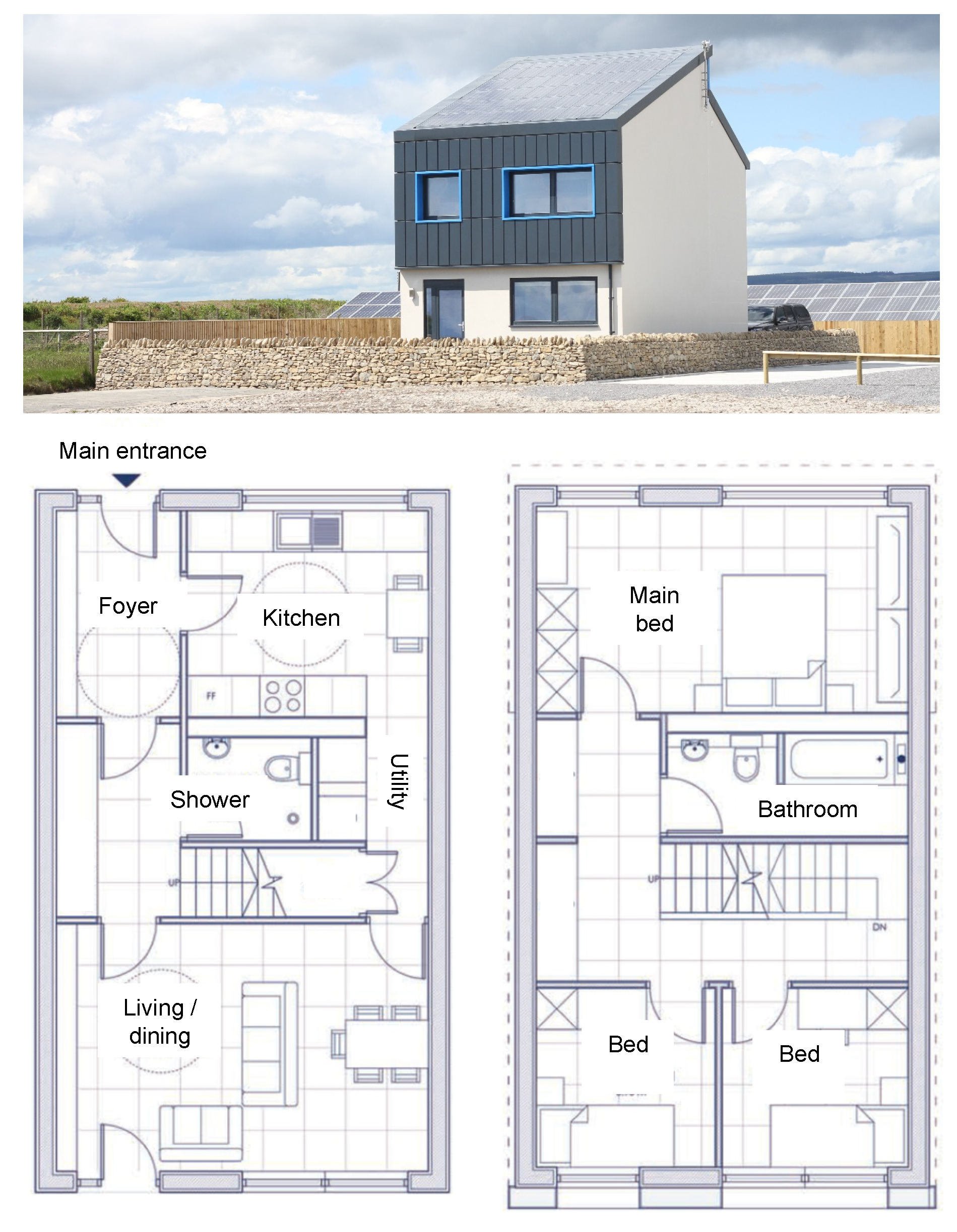
The SOLCER house is a three-bedroom detached house of 100 m² floor area, intended for the social housing market (Figure 2). Although the house is detached, it would normally form part of a semi-detached or terraced development. The design of the SOLCER house used a number of technologies and design approaches that were developed through the Low Carbon Research Institute (LCRI) Low Carbon Buildings Programme [38]. These have been optimised using a systems approach, through two stages of integration. Firstly, the electrical and thermal technologies were integrated, with solar PV and battery storage powering a heat pump, combining with a transpired solar (thermal air) collector (TSC) and mechanical ventilation heat recovery system (MVHR), to provide space heating and domestic hot water (DHW). The solar PV and battery storage also provide power for lighting and electrical appliances. Secondly, the energy systems were integrated into the building design, with the PV panels as the south-facing roof, and the TSC as the external south-facing, first-floor external wall finish.

The architectural design and construction of the house was carried out by Cardiff University. The house was designed based on available technology and using local supply chains. A major design criterion was affordability, and the estimated cost of replication at the time of construction was £1200/m² of usable floor area, which was considered comparable to the then-current social housing costs (2015).

2.1. Building Design for Reduced Energy Demand

The energy demand of the house was reduced to a near ‘Passivhaus’ level [39]. However, the design did not follow the Passivhaus standard rigorously, in order to allow the use of technologies and local suppliers that may not be compliant with Passivhaus accreditation requirements. The house was designed to have high levels of thermal insulation and a low air leakage. The house used a structural insulated panel system (SIPS) method of construction with 172 mm of climate EPS insulation contained between two layers of oriented strand board (OSB). The windows were double-glazed timber frame, with an aluminium external finish. The thermal insulation levels for the main design elements are summarised in

Table 2. Thermal insulation levels for the main design elements with building regulation values for comparison.

Element	W/°C/m2
	SOLCER House	Welsh Building Regulations [40]
Wall U-value	0.12	0.21
Ceiling U-value	0.10	0.15
Floor U-value	0.15	0.18
Window U-value	1.12–1.51 *	1.60

* Depending on window dimensions.

. The south-facing roof comprises of a large (34 m² area) solar PV panel, which is fully integrated into the design of the building, with the southerly roof space, naturally lit through the transparent areas around the PV cells. This approach provides a different aesthetic, and potentially reduces costs, compared to a solar PV system ‘bolted-on’ to a standard roof. The north-facing roof is constructed from an SIPS panel with a standing seam metal cladding external finish.

The south-elevation first-floor of the house incorporates a transpired solar collector (TSC) with an area of 14 m², which is used to collect solar thermal energy, preheating the incoming ventilation air to the building to supplement space heating. External air enters the TSC through a grid of small (1 mm²) holes in the metal cladding. These systems were previously investigated as part of the LCRI Low Carbon Buildings Programme [38].

The building is modular in its design, based on a 0.6 m by 0.6 m dimension grid. The whole building took sixteen weeks to construct, taking place during the mid-winter period. The house is located at the Cenin ‘energy cluster’ industry park in South Wales, where there is a range of renewable energy generation systems, including solar PV, wind and anaerobic digestion. The house is used as a test facility and is currently fully occupied as an office and meeting space.

2.2. The Design of the Energy Systems

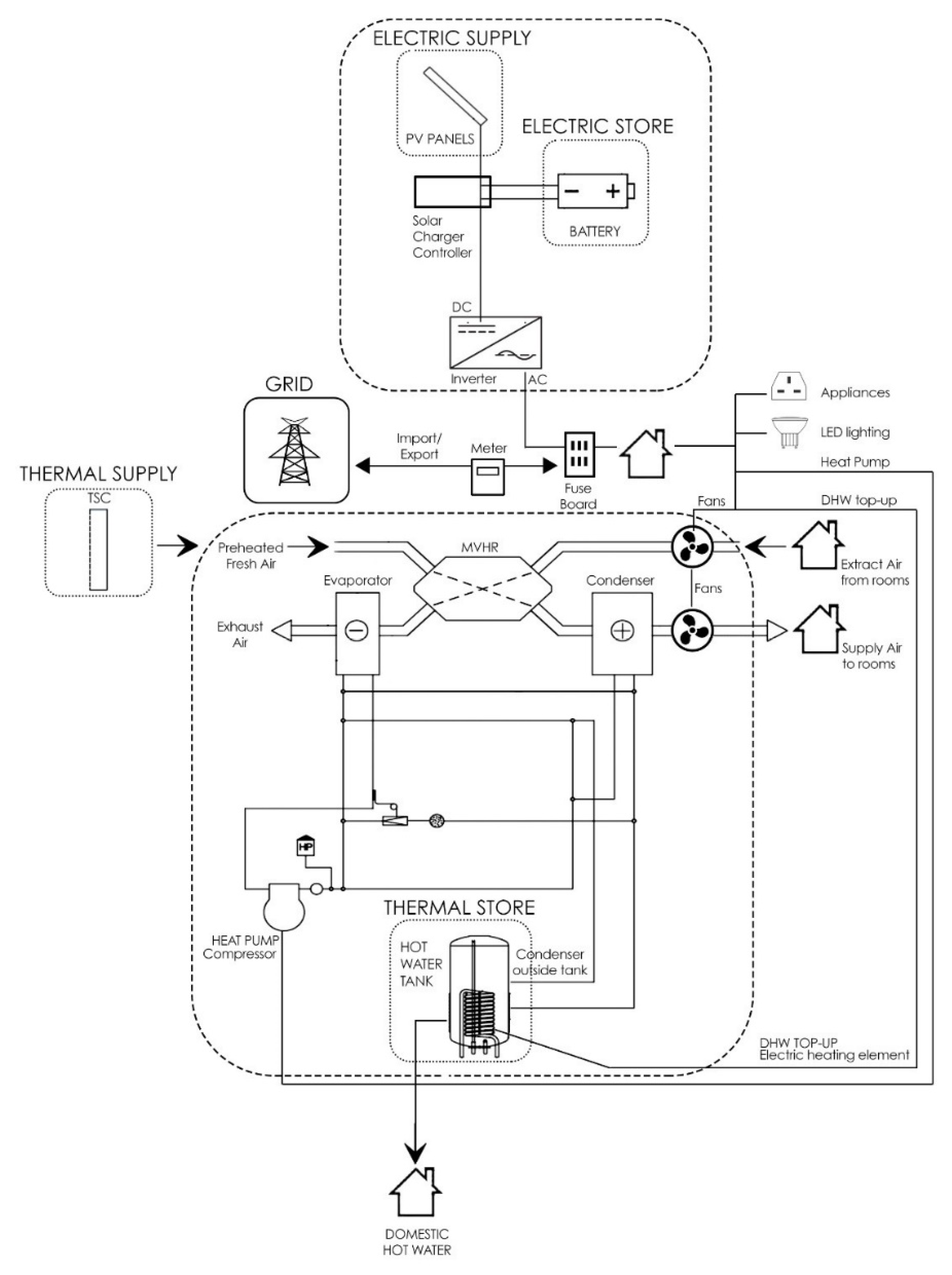
Figure 3 presents a schematic of the SOLCER house’s electrical and thermal system. The energy supply is all electric, providing space and domestic hot water heating and powering electrical appliances. The 34 m² solar PV array has a capacity of 4.3 kWp. This is combined with a 6.9 kWh lithium-ion-phosphate Victron battery, which is located within the roof space. The battery and PV array are connected via a DC-coupled system, which is connected to an inverter to provide AC power to the house. The backup grid supply connects into the AC circuit. The PV and battery storage system provide power to the ring-main, LED lights and the heat pump and mechanical ventilation system. Electricity is drawn from the grid when there is insufficient power available from the PV and battery system. The aim is to maximise the use of the renewable energy within the house, and only export to the grid when all the house energy needs are fulfilled.

The thermal system comprises a transpired solar collector (TSC), mechanical ventilation with heat recovery (MVHR) integrated with an exhaust air heat pump and a thermal water store. This system provides space heating through the ventilation, with fresh air supplied mechanically to the main living spaces and extracted from the kitchen, bathroom and shower room. The building has a low heat demand and so can be heated through the ventilation system. For space heating, external air enters the TSC and is preheated from incident solar radiation, when available. The air then passes through the heat exchanger of the MVHR and then, if necessary, is topped up with heat by the heat pump. Exhaust air leaves through the MVHR, exchanging heat with the incoming supply air. It then passes to the evaporator of the heat pump, which heats both supply air and the thermal water store. The heat pump collects heat from the exhaust air, which is at internal air temperature (minus the heat exchanged through the MVHR), thus maintaining a relatively high coefficient of performance (COP) over the heating season. The exhaust air therefore can be considered to contribute to the space and DHW heating through the operation of the heat pump. When space heating is not required during warmer weather, the TSC and heat recovery stages are bypassed, and the MVHR acts solely as a mechanical ventilation supply air system. The heat pump is powered either from the solar PV coupled to battery system, or from the grid when there is no direct PV solar supply and the battery is exhausted. The MVHR, heat pump and thermal store are all contained within the single Genvex Combi 185LS EC unit. The thermal system details are presented in

Table 3. Specification of thermal system (design values).

TSC	Area	14.0 m2
MVHR	Flow rate (manufacture’s value)	42 L/s (150 m3/h) *
Heat Pump	Capacity COP (manufacturer’s seasonal value)	585 W (max) (average 425 W) 3.21
Thermal store	Volume	185 L

* Different values for flow and return were measured in practice (as described in Section 4.1). COP: coefficient of performance.

.

The house has been continuously monitored on a 5 min interval, using the equipment using the sensors detailed in

Table 4. Specification of monitoring equipment.

Data Collection	Equipment	Resolution
Mains grid electricity import and export.	Elster A100C.	Single-phase meter with pulsed output and with reverse energy flow for import/export.
Submetering of electricity demand.	YTL DDS353 45amp.	Single-phase meter with a single-pulse output and LCD screen.
Temperatures.	Eltek DD47 transmitters connected to an Elteck SRV250 receiver logger and 3G connectivity.	Temperature resolution of 0.1 °C (±0.4 °C at −5 to 40 °C)

. The monitored data have been used to make comparisons with simulations at component and whole house scale.

3. Building Energy Modelling: System Component Testing

Energy modelling was used both in the design of the building and in the evaluation of its performance. During the design stage, the solar PV and battery storage were initially sized using the buildings as power stations (BAPS) tool, which was developed during the early design stages to predict the balance between energy demand reduction, renewable energy supply and battery storage [41]. However, for performance evaluation, a more detailed building energy model was needed to simulate the whole house performance, including all the elements of the heating and ventilation system. The analysis of the energy design was carried out using the building energy model, HTB2 [42], with external plugins to simulate specific components of the energy system. This model is able to simulate the annual hourly thermal performance of the building, using local weather data, building construction details and occupancy profiles. HTB2 has been developed at Cardiff University over a period of nearly 40 years, and has undergone extensive testing and validation, including the IEA Annex 1 [43], IEA task 12 [44] and the IEA BESTEST [45].

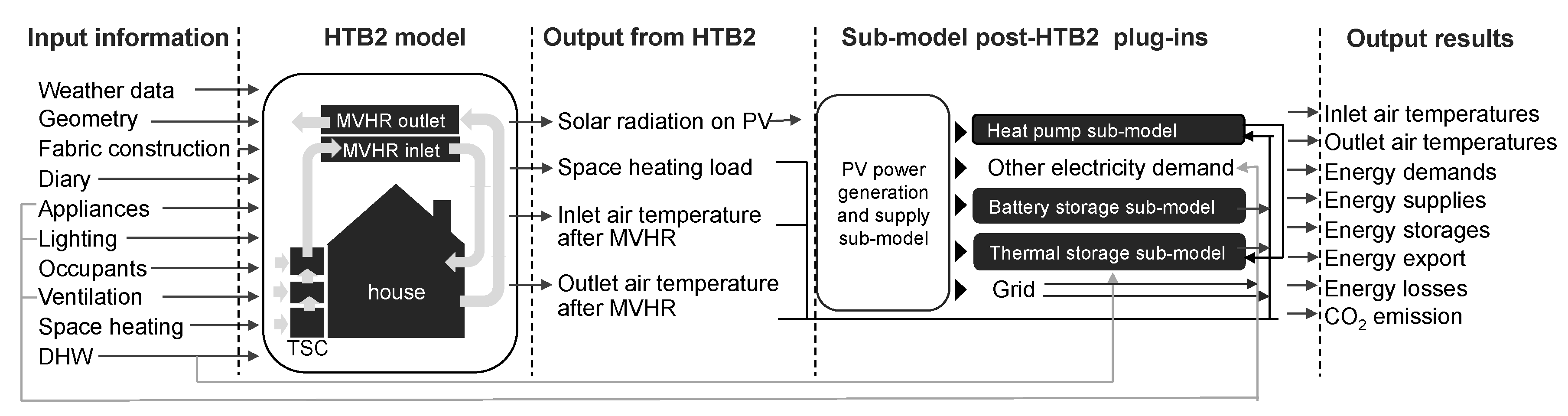
The thermal and energy system components of the SOLCER house have been added to the model, either through submodels within HTB2 (for the MVHR and TSC), or through separate ‘plugin’ submodels operated at the post-processing stage (for the heat pump, battery, thermal storage), as illustrated in Figure 4. This has resulted in a ‘bespoke’ version of HTB2, specifically set up for modelling the SOLCER house. The modelling framework for the thermal and electrical system is summarised below.

3.1. Transpired Solar Collector (TSC)

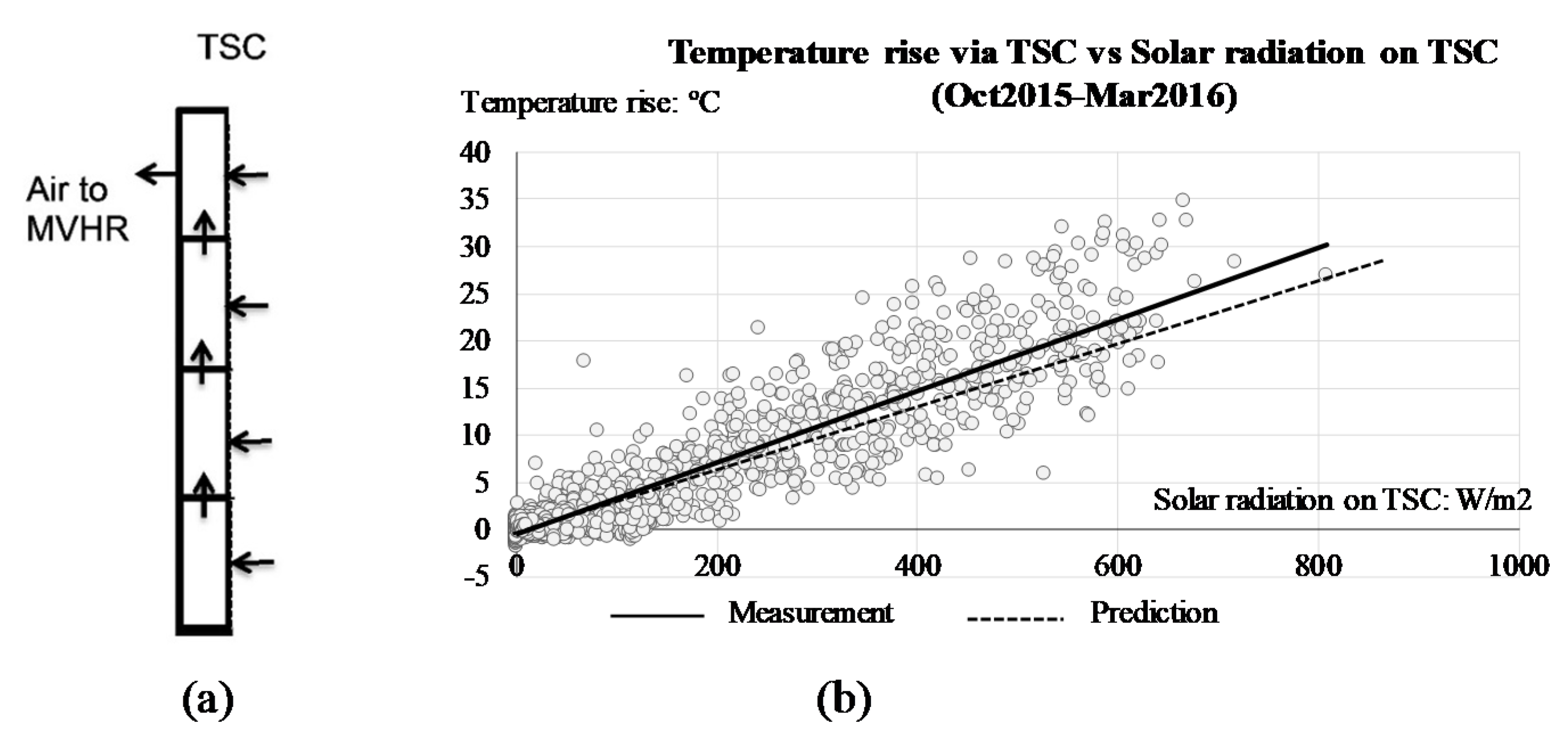
The TSC is modelled as four vertical spaces within the HTB2, one above the other, as shown in Figure 5a. External air enters each space and air passes upwards through the higher spaces until it is extracted from the top space and fed into the MVHR submodel. The total amount of input air is divided equally across the four spaces of the TSC. The TSC submodel simulations have been compared to measured data from the SOLCER House for the air temperature rise between the inlet (external air temperature) and the outflow of the TSC for the heating season (Figure 5b). There is reasonable agreement between the simulated hourly values and the average measured data, indicating that the TSC submodel is providing a realistic simulation. It has been suggested [46] that the relatively warm external air boundary layer of the TSC provides a useful contribution to the overall energy performance, in addition to the transfer of heat from the solar-heated metal surface in the TSC cavity. This might account for the small under-prediction (generally around 1 °C) compared with the measured results. The relative high exposure of the site to wind may also reduce the external boundary heat-gain. The TSC can deliver in excess of 20 °C rise in air temperature to the incoming air (for an incident solar radiation level of 600 W/m²).

3.2. Mechanical Ventilation Heat Recovery (MVHR)

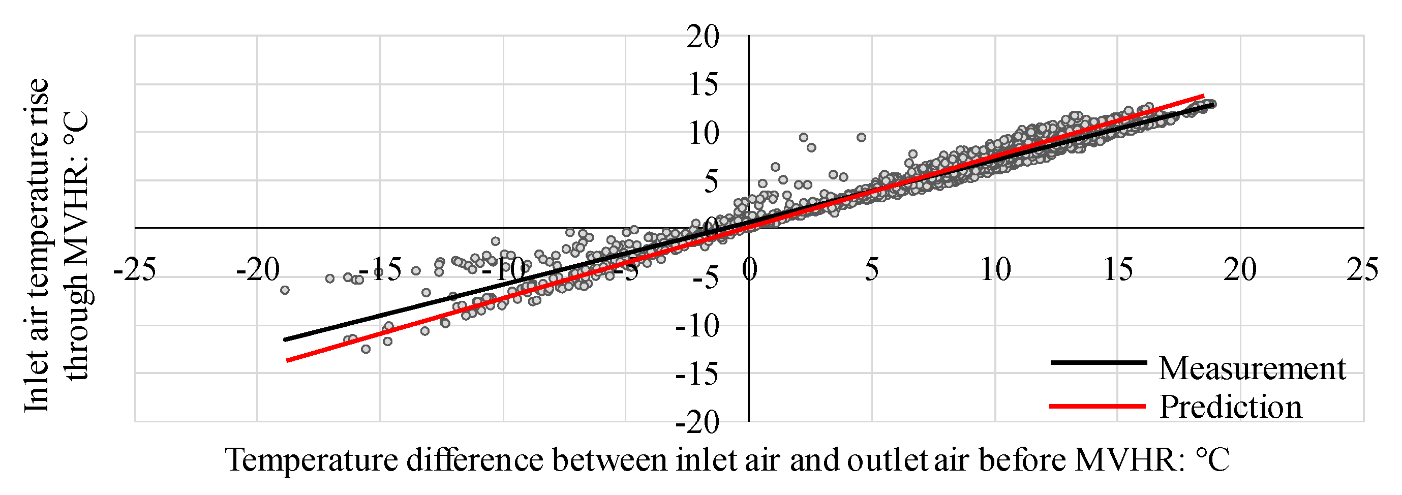
The MVHR has been modelled within the HTB2, using two spaces, one a path for the supply air and the other a path for the exhaust air. The spaces share a common metal ‘wall’ with a surface area equal to the sum of the heat exchange plate areas of the MVHR unit. A plate-surface heat transfer coefficient of 72 Wm⁻² K⁻¹ was selected as an appropriate value for airflow through a narrow cavity [47]. HTB2 then simulates the hourly heat exchange between the exhaust air and the supply air. The results of the MVHR simulation are compared to measured data in Figure 6. The temperature rise through the MVHR of incoming air is plotted against the difference between the inlet and outlet air temperatures. The agreement between measured and predicted results is good with a maximum difference of around 1 °C at the extremes of operation.

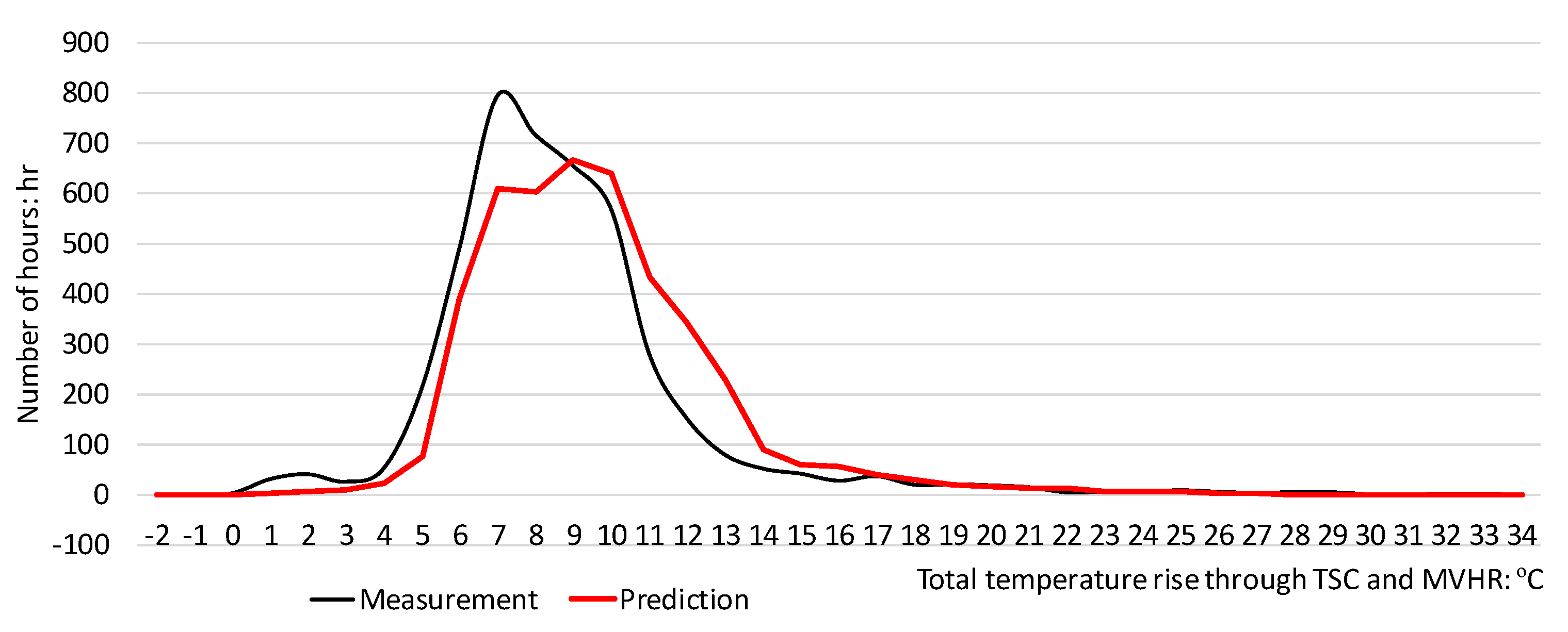
The performance of the TSC linked to the MVHR is presented in Figure 7, as an hourly distribution of temperature rise, comparing predicted with measured data. The results imply that the level of fit between measured and predicted data is such that the model can be reliably used to assess the overall performance of the house with respect to the combined elements of the TSC and MVHR. The measured inlet and outlet flow rates were different from the manufacturers values (Table 3). For the year 2015/6, the average flow rates were 41 L/s for the inlet and 31 L/s for the outlet, implying an over -pressure mode of operation. The measured rates were used in the simulation for the office situation in Section 4.

3.3. Exhaust Air Heat Pump

The heat pump supplies heat as required to the incoming air for space heating, and for heating the thermal water store. The manufacturers stated COP value of the heat pump is 3.21 (Table 3). The electricity needed to operate the heat pump is predicted on an hourly time-base for space heating, calculated by HTB2, and for hourly DHW demand, based on occupancy use. The DHW temperature is calculated based on its storage capacity, the use pattern and cylinder losses. When the predicted temperature of the water in the thermal store falls below 50 °C, the heat pump operates to raise the water temperature to a maximum 52 °C.

The Genvex Combi unit has an evaporator coil and two condensing coils. One condensing coil is used for heating DHW, and the other for space heating. The unit’s controls are set to prioritise either heat for DHW or for heating the supply air for space heating. It cannot do both simultaneously. The default setting prioritises DHW. However, the user can change the priority to space heating if required. Once the DHW tank is up to temperature, the unit will automatically switch to space heating, if it is required. If there is no demand for heat, the heat pump will switch off, but heat recovery through the MVHR will continue.

3.4. Thermal DHW Store

The thermal DHW store is activated between a temperature of 52 °C and 65 °C. The heat pump raises the DHW temperature to 52 °C, when it requires heat input. When excess solar PV electricity is available, after the demand from the heat pump, small-power-demand battery storage is met; it will be used to heat the DHW. It will raise the DHW temperature up to a maximum of 65 °C. The temperature required to eliminate Legionella bacteria is 60 °C, and if it is not met by PV electricity once a week, an electric immersion heater will operate. The DHW storage tank heat loss is calculated considering its thermal insulation.

3.5. Solar PV and Battery Storage, Inverter and Grid Electricity Supply

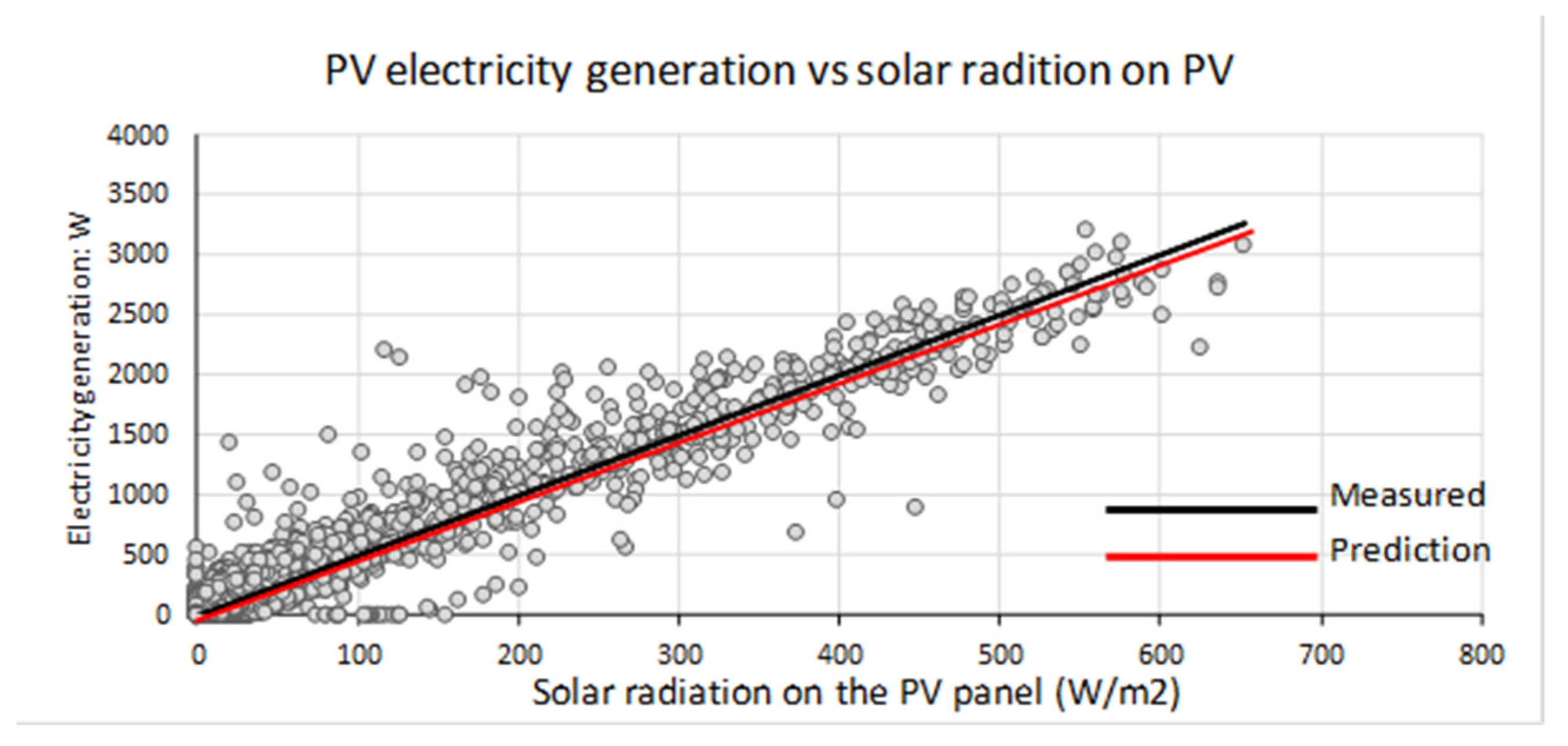
The solar PV array is simulated within the HTB2 from the predicted hourly solar radiation incident on the PV surface. A module efficiency of 15% was applied to the simulated incident solar radiation. The cell efficiency in standard test conditions (STC) is 19.6%, but this is reduced due to the spaces between cells in the module panel and the panel frame. The battery is allowed to discharge down to 20% of its capacity; discharging below this is detrimental to the lifetime of the battery. Figure 8 compares the measured and predicted PV energy generation for the second year of monitoring. The average measured value of 15.6% compares well with the manufacturers value of 15%.

4. Model Testing

The previous section described the modelling set up for ‘the HTB2 and its plugins, and showed that when simulated data was compared to measured data on a component basis, there was generally a good correlation. In this section the whole-building performance simulation results are compared to the measured results for the SOLCER house when used as an office, which is the real-life situation. SOLCER was used as a test house and so did not have a normal residential occupancy. The hours of occupation were office hours from Monday to Friday. The results from the simulation are compared with the measured data. However, as described below, the initial heating season (October to March) energy simulation results were different from the measured data. On investigation this ‘performance gap’ was attributed to a range of factors, which are discussed below.

4.1. Performance Gap

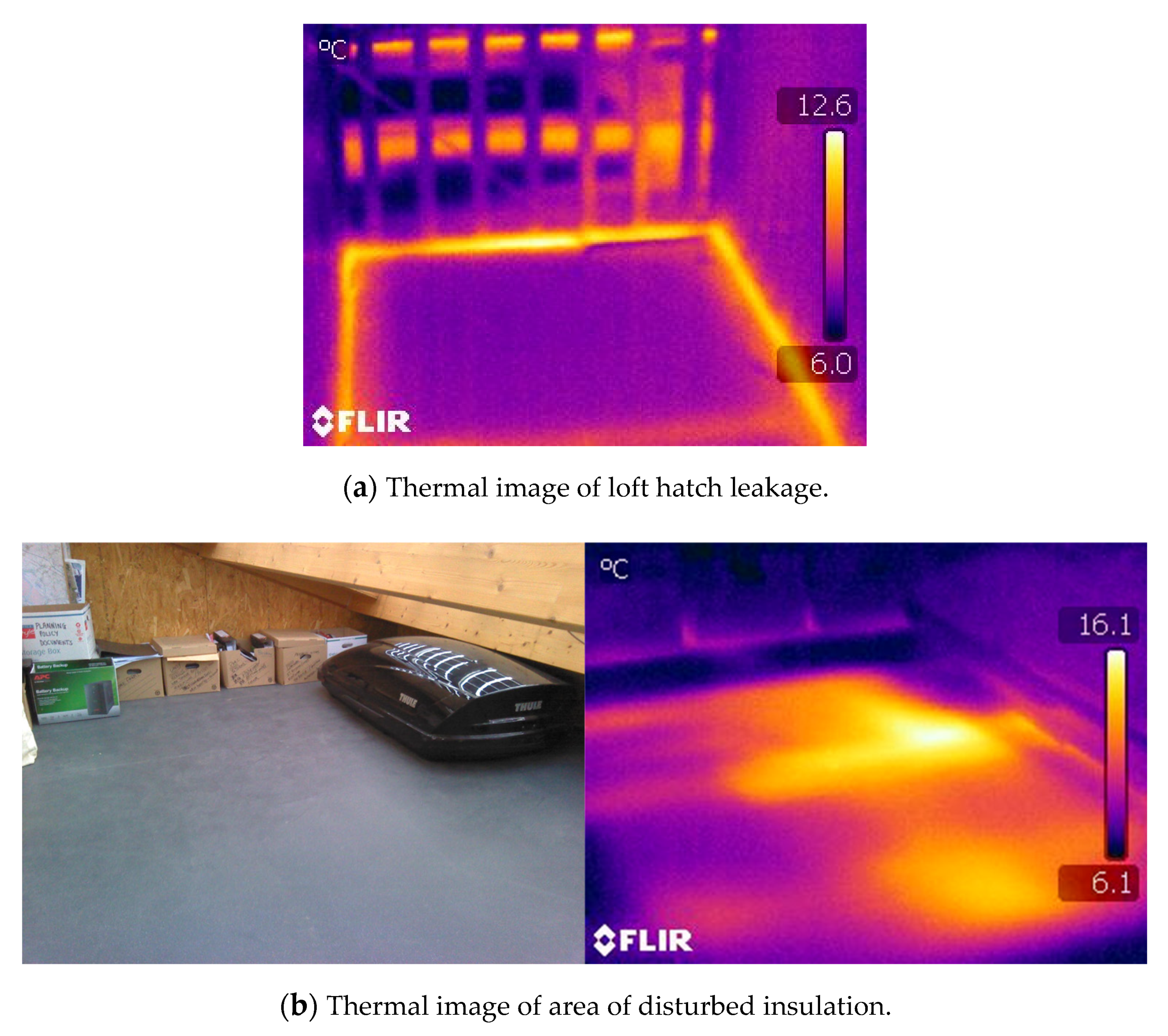
The measured total heating energy was 4732 kWh for the heating season 2015/16 (

Table 5. A summary of the heating performance adjustment for the simulation accounting for the performance gap (kWh).

Heating October 2015–March 2016	Measured Annual Heating Energy	Initial Simulated Annual Heating Energy	Loft Air-Leakage Adjustment	Secondary Causes Adjustment	Simulated Annual Heating Energy after Adjustments
	4732	1749	+1422	+820	3991

). This value compares to the initial simulation result of 1749 kWh. There was therefore a significant difference of nearly 3000 kWh between the measured data and the simulation results, which would increase the annual heating costs by an estimated £140. Of course as the energy demand of a building is reduced, the performance gap will become of greater significance and a percentage of annual energy use. A number of reasons were identified to account for this performance gap. A main contribution to the performance gap could be the air leakage to the loft through the loft hatch, which was initially identified through a thermographic survey as leaky (Figure 9a), during a ‘blower door’ pressure test, which measured the air leakage 2.91 m³/h/m² at 50 Pa. When this was accounted for, the predicted heating energy consumption rose from 1749 kWh to 3172 kWh. There were also a number of secondary causes identified. The insulation between the main space and the roof space had been disturbed during construction, which was identified through a thermographic survey (Figure 9b). Measurements of the air supply and extract to and from the spaces were different to the manufacturer’s data (the measured supply was 41 L/s and extract 31 L/s, compared to a balanced supply extract of 42 L/s). When all factors were considered, the adjusted simulation heating demand rose to 3991 kWh which is 16% lower than the measured demand. However it should be recognised that the building will not always be operated the same throughout the period, which would also contribute to the performance gap. Also, the computer model itself, although having the checks carried out in Section 3, will have inherent inaccuracies due to assumptions made. However, this performance gap analysis illustrates the need for in-construction checks, so that deficiencies can be immediately corrected during the construction process.

4.2. Annual Simulation

With the above adjustments made to the simulation, accounting for the performance gap, the simulations and measurement comparisons for the house as used for office activities were carried out for the heating season October 2015 to March 2016.

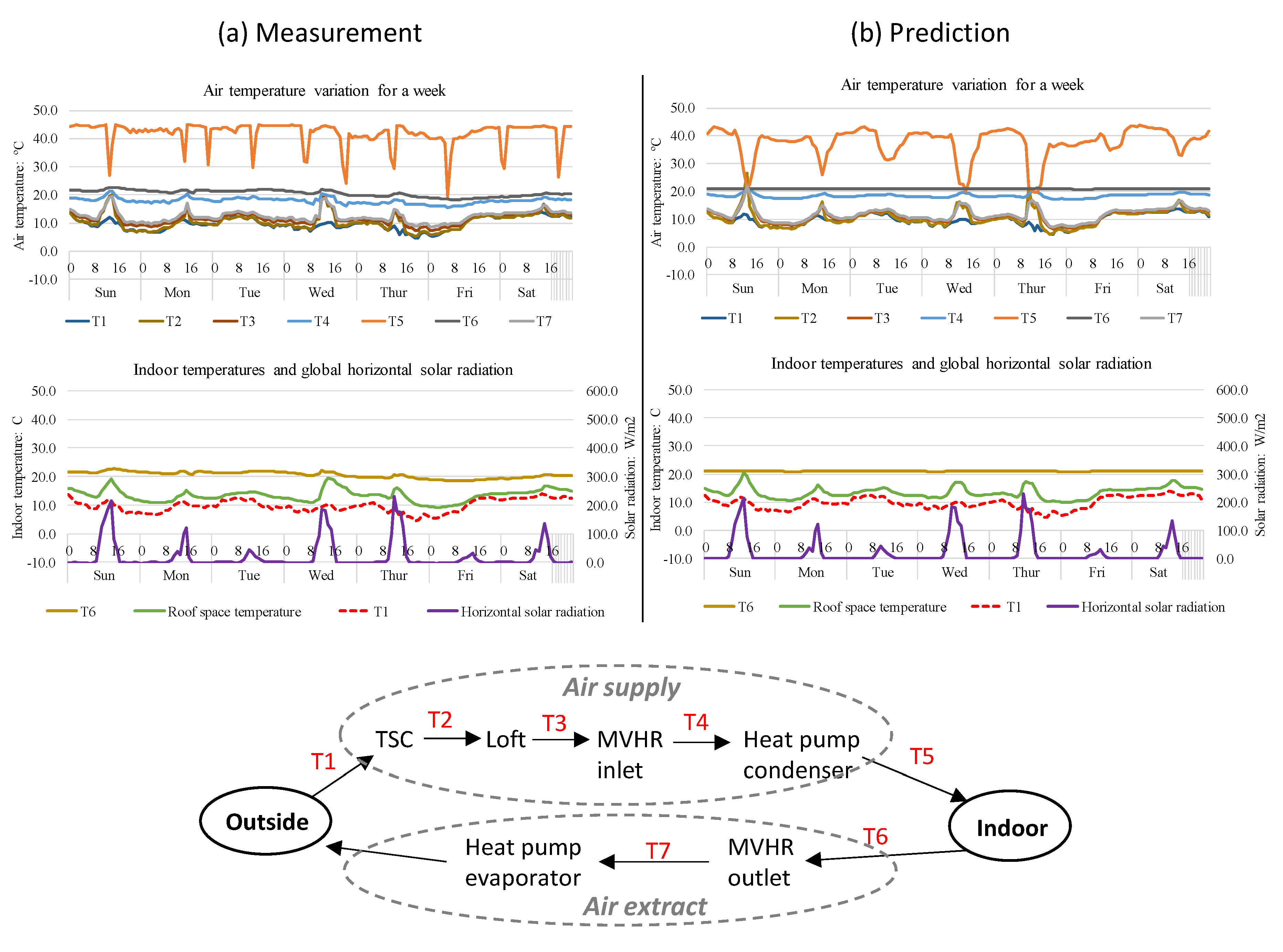
The HTB2 was run for the typical heating period. Measured data and simulation results are compared for an example week in December 2015, which is presented in Figure 10. There are two pairs of graphs, the upper plotting the air temperatures through the heating and ventilation system and the lower plotting the space and external air temperatures and the horizontal solar radiation. These plots are included to illustrate the detailed level of the simulation and the relatively good agreement of predictions with measured data. For example, the results show the effect of solar heat raising the air temperature through the TSC, the heat gain of the supply air through the MVHR and the close comparison of the roof space modelled and measured data, the latter accounting for the increased heat loss to the roof space due to loft hatch air leakage and disturbed ceiling insulation.

Table 6. A summary of predictions against measured data for the heating period and the selected example week (kWh).

Period	Measurement or prediction	Heat Gains by TSC	Heat Loss by TSC	Heat Gain by Loft Inlet Duct	Heat Loss by Loft Inlet duct	Heat Gain by MVHR	Heat Loss by MVHR	Heat Delivered by HP	Heat Delivered by Electric Heater	Total Heat Delivered
October 2015–March 2016 (in kWh/season)	Measurement	446	−13	342	−37	1399	−41	3911	821	4732
	Prediction	504	−20	275	−70	1491	−80	3991	0	3991
7 day period December 2015 (in kWh/week)	Measurement	6.5	−0.4	10.3	−0.1	50.9	0.0	197.4	−8.3	189.1
	Prediction	6.7	−0.6	7.9	−0.9	56.2	−0.1	172.5	0	172.5

presents the energy performance of the various components over the heating season and for the example December week. The results for the predicted heating energy performance is 3991 kWh for the 2015/16 heating season, and 172.5 kWh for the example week. This compares to measured values of 4732 kWh and 189.1 kWh for the heating season and example week respectively. As one might expect the comparison is closer for the example week, where operating conditions and control settings are relatively stable, than for the heating season, where occupancy and control settings may be more variable. The table presents the heating season heat gains and losses throughout the air system, for the TSC, the loft exposed insulated ductwork that connects the TSC to the MVHR, the MVHR and the heat supplied through the heat pump. It also presents the direct electric heater load, which comes into use if the heat pump cannot meet the load by itself. This is not included in the simulation as the heat pump alone is assumed to provide the ‘top-up’ load.

5. Modelling Results for Domestic Use

In this section the simulation model (HTB2 plus plugins) is used to explore the SOLCER house performance under typical simulated domestic occupancy conditions, assuming the building performs as designed in relation to air leakage and mechanical ventilation inlet and extract flow rates (as specified in Table 3) and the performance gap has been rectified.

5.1. Heating and Electrical Loads

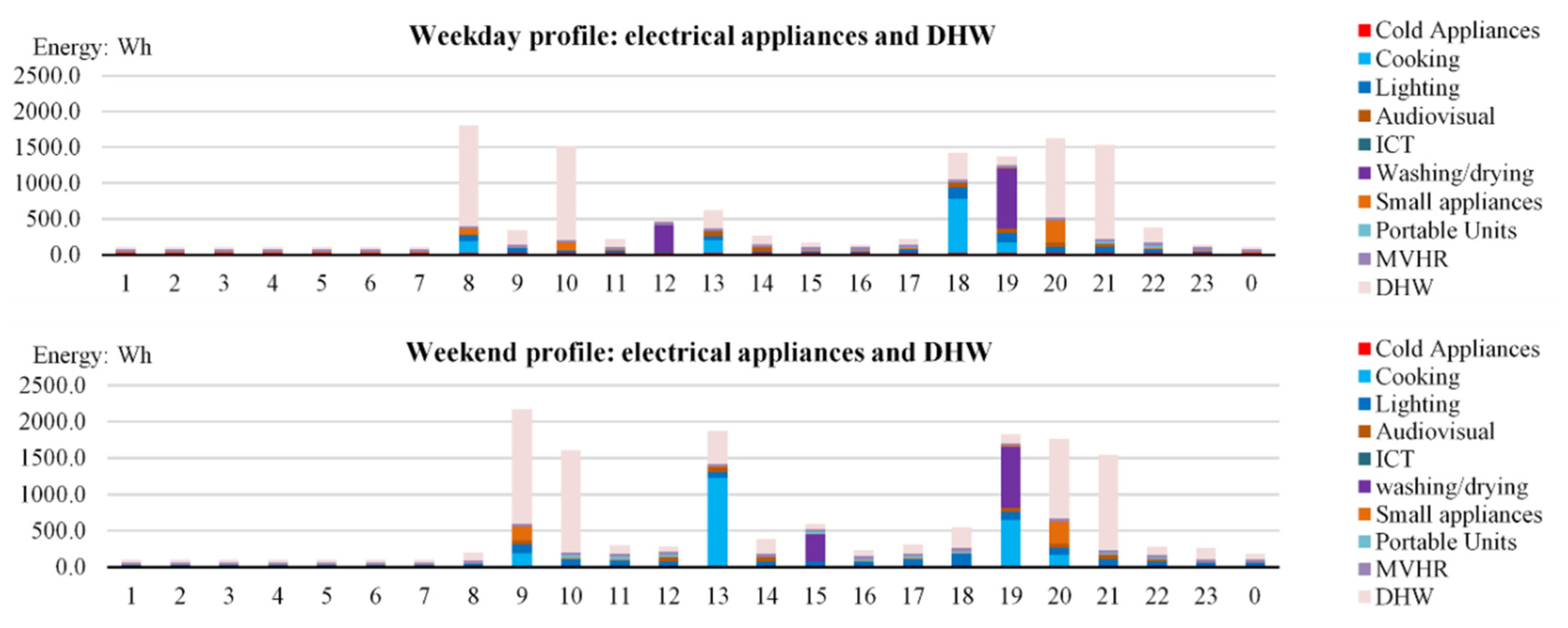
The heating and electrical loads are based on a typical domestic occupancy pattern. An occupancy profile of energy use was set up for a typical weekday and weekend. The electricity demand was estimated from hourly use profiles for appliances and lighting appropriate for an adult couple with two children, plus the electricity used for the heat pump and TSC/MVHR fan system (

Table 7. Electricity and domestic hot water (DHW) system capacities and demands.

Demand	Capacity (W)	Daily Use (kWh/day)–Weekday/Weekend
Lighting	-	1.0/1.3
Small power	-	4.1/5.3
Heat pump	585	0–8.9
Fans	71	0.9
DHW	-	6.3/6.9 (weekly average of 150 L/day) (not including storage and distribution losses)

). The electricity usage profile is based on a published survey [48], applied for an adult couple with two children occupying the house. Hourly hot water use profiles for the household were based on existing data [49]. For the purpose of this exercise, it was assumed that one of the adults works full time, while the other stays at home to take care of a younger child, while an older child attends school every weekday. From this data typical daily profiles were created and are presented in Figure 11.

The results of the building energy modelling are presented in the following sections for:

(i)

Typical daily temperature and energy profiles (Section 5.2).

(ii)

Annual Energy performance (Section 5.3).

(iii)

Analysis of the performance of the TSC and MVHR contribution to the energy performance (Section 5.4).

(iv)

Analysis of variations in energy demand of electrical appliances and DHW usage (Section 5.5).

5.2. Daily Temperature and Energy Profiles

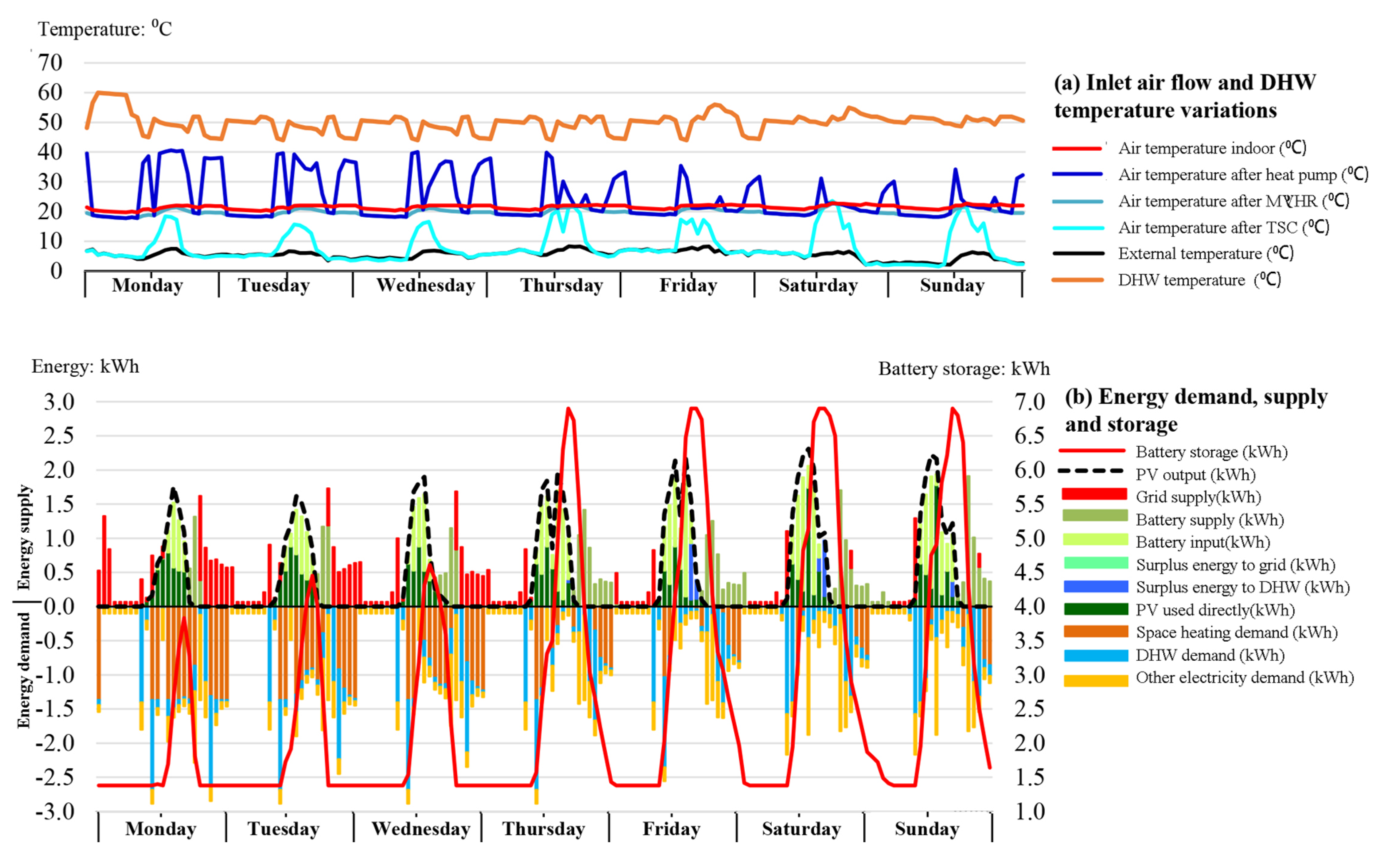
Figure 12a presents simulated temperature data during a winter ‘sunny’ week, for the air as it travels through the ventilation system, for a relatively sunny winter week. The TSC adds a significant amount of heat during the sunny period, which boosts the air temperature up to 20 °C. For an overcast condition, the MVHR still can boost the air temperature by up to a 17 °C temperature rise. The air is supplied to the space at around 40 °C. Figure 12a also presents the DHW temperature in the cylinder When there is a DHW heating demand the heat pump switches from space heating to DHW heating, which can be observed through the drop in supply air temperature. An analysis of the simulated solar PV generation and grid energy supply is presented in Figure 12b, alongside the battery storage, and the various thermal and electrical demands. As the PV power generated during a sunny day is able to meet the majority of energy uses, power from grid is only imported during some nighttime or early morning periods.

Figure 13a presents the simulated indoor air temperature data for a summer ‘sunny’ week, showing it peaking at between 23 °C and 26 °C, which indicates that overheating is not a major issue (this was supported by on-site measurements). The TSC can be bypassed in summer, and the MVHR changes to the summer mode, just supplying fresh air to the main living spaces with no heat recovery. Figure 13b provides a detailed analysis of the simulated solar PV and grid energy supply, alongside the battery storage, and the various thermal and electrical demands. During this period, the PV power is able to supply all the building energy needs, and so no power is imported from grid. Also, the PV system exports some 50% of electricity to the grid.

5.3. Annual Energy Performance

Table 8. Summary of monthly and annual energy demand, supply and carbon dioxide emissions.

	Energy Demand (kWh)							Energy Supply to House (kWh)				Others (kWh)		CO2 Emissions * (kg)
	Space heating demand	DHW demand	Heat pump	Electric air heater	Immersion heating	Other electrical	Total electrical	PV output	PV used directly	Battery supply	Grid supply	Surplus PV energy to grid	Total losses	Due to power import	Due to power export	Net carbon
January	376	223	179	12	13	197	401	142	89	49	262	0	3	136	0	136
February	279	202	132	22	36	179	369	223	104	80	166	7	14	86	−3	83
March	199	224	114	6	52	199	371	340	127	94	105	57	17	55	−30	25
April	33	217	53	0	80	193	326	499	129	97	22	176	19	11	−91	−80
May	0	223	34	0	115	197	346	647	141	90	7	291	16	4	−151	−148
June	0	217	34	0	109	193	336	594	147	79	3	247	14	1	−128	−127
July	0	224	31	0	125	199	355	672	153	76	1	305	13	0	−158	−158
August	0	223	33	0	117	197	347	592	138	93	1	230	16	1	−119	−119
September	0	217	43	0	80	194	317	442	111	112	18	125	17	9	−65	−56
October	8	223	61	0	36	197	295	270	91	104	65	20	20	34	−10	23
November	210	216	130	1	9	191	330	159	87	59	181	1	9	94	0	93
December	359	224	174	14	11	200	399	122	83	33	283	0	6	147	0	147
Annual	1464	2634	1016	54	782	2339	4191	4701	1401	966	1112	1458	165	577	−757	−179

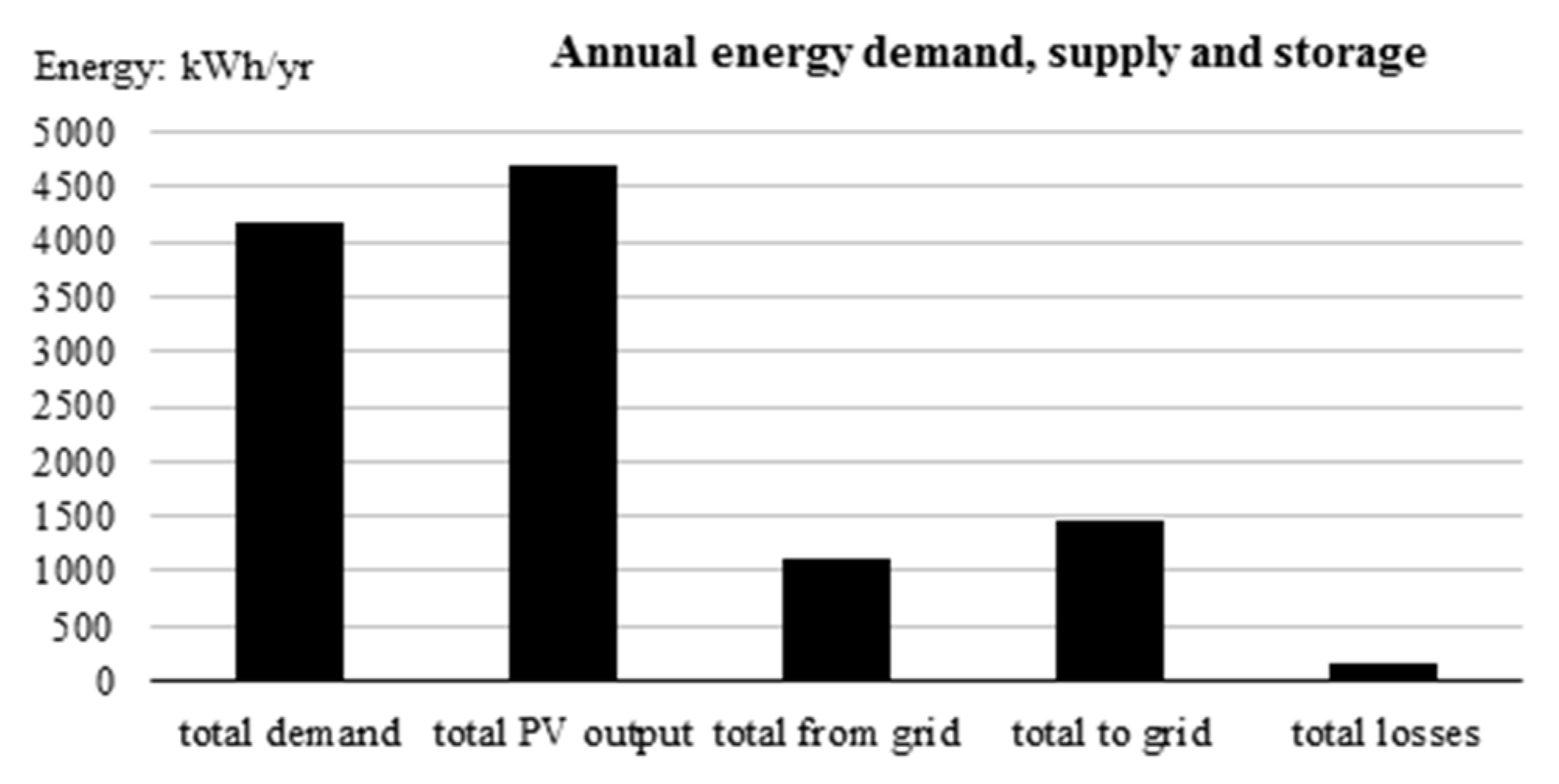
* The operating carbon emissions are calculated using an emission factor of 0.519 kg CO₂/kWh for electricity [50].

presents a summary of the predicted monthly and annual energy demand, energy supply and carbon dioxide emissions for the domestic scenario. The space-heating load is relatively low (1464 kWh), compared with the initial simulated results for the office scenario in Table 5 (1749 kWh), however, the occupancies are different. Table 8 shows that the annual DHW heating load is considerably higher than the space heating load, given that the space-heating load occurs only over the heating season. The total heating demand from space-heating and DHW is 4098 kWh (that is 1464 + 2634). The energy supply to meet that demand is 1016 kWh from the heat pump plus 782 kWh from the electric immersion heater. There is an additional 54 kWh used for the direct electric top-up heater located in the air supply after the heat pump, which is operated at times when the heat pump cannot provide to total heating demand. The total energy supply for space-heating and DHW is 1852 kWh. The electricity used for domestic appliances and lighting is 2399 kWh. Based on the break down above, the total annual electricity used by the house is 4191 kWh. Of the 4701 kWh energy generated by the solar PV system, only 1401 kWh is used directly in the building as it occurs, with the battery storage extending this use by a further 966 kW. The losses of 165 kWh are mainly attributed to battery charging and discharging efficiency losses. There is a negative net CO₂ emission of −179 kg per year associated with the house. The total annual electricity imported from the grid is 1112 kWh compared to the exported value of 1458 kWh, indicating the energy-positive performance of the house by 346 kWh, so the export to import ratio is 1.31. The annual energy performance is summarised in Figure 14.

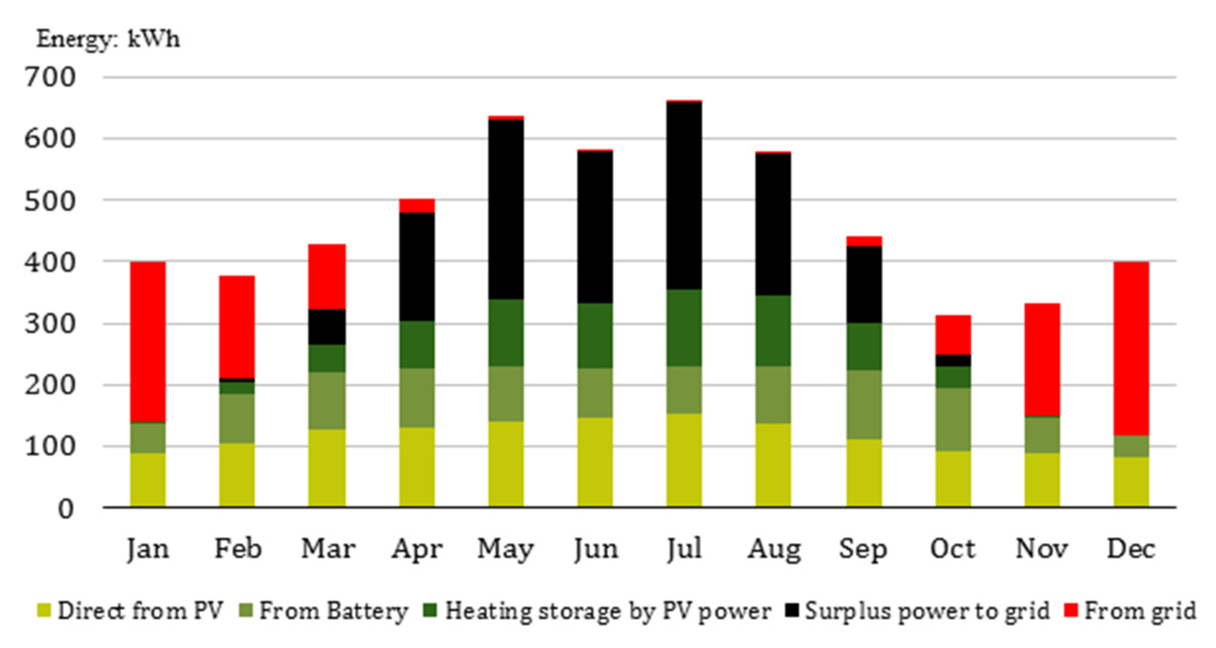
Figure 15 presents monthly values of energy for the PV and battery supply, grid supply and PV export to the grid. It shows that the energy imported from the grid peaks during the winter period, and the PV energy exported to the grid peaks in summer. The surplus power exported to the grid exceeds the power imported from the grid.

5.4. Analysis of the TSC and MVHR Energy Performance

Further investigation has been carried out to examine the benefits gained from adding the TSC and MVHR to the thermal system [51]. Cases without the TSC, and the TSC with and without the MVHR were simulated (

Table 9. Performance predictions of cases with and without TSC and/or MVHR.

Cases	Heating by TSC (kwh)	Heating by MVHR (kwh)	Space Heating Demand (kwh)	The Contribution of TSC and MVHR to Space Heating (kWh)
With both TSC and MVH	682	3605	1464	74.5%
Without TSC	n/a	4106	1534	72.8%
Without MVHR	682	n/a	3814	15.2%
Without both TSC and MVHR	n/a	n/a	4267	0%

). The TSC alone contributes some 15.2% to the heating. The MVHR on its own contributes some 72.8% to the heating. The combination of the TSC and MVHR contributes some 74.5% to the heating. It is also illustrated that the performances of the TSC and MVHR conflict to a certain extent. The results question the cost-effectiveness of the TSC in this configuration. It would be beneficial if the TSC heat could be used to contribute to DHW heating during the summer period.

5.5. Analysis of Energy Demand of Electrical Appliances and Dhw Usage

The house has been simulated for a range of scenarios for electrical appliance and DHW usage, considering the available energy-efficient and water-efficient products on the current market. The results are summarised in

Table 10. Performance prediction of different scenarios.

Case	Scenario		Self-Sufficiency	Surplus Power Export/Power Import
	Electrical Appliances Demand	Domestic Hot Water Demand
Base case	2339 kWh/y Current energy-efficient scenario based on the most energy-efficient products available in the market.	150 L/day Published survey sample [49]	73.5%	1.31
I	3245 kWh/y Published survey sample for household with children [48]	150 L/day Published survey sample [49]	71.5%	0.70
II	2662 kWh/y Improved energy-efficient scenario compared with case I [48]	150 L/day Published survey sample [49]	74.1%	1.01
III	2662 kWh/y As above	129 L/day Published survey sample [49] + available water-efficient products in the market	74.4%	1.12
IV	2339 kWh/y Current energy-efficient scenario based on the most energy-efficient products available in the market.	129 L/day Published survey sample [49] + available water-efficient products in the market	73.9%	1.43

Note: For case IV and the current base case, the energy-efficient and water-efficient scenarios are developed referring to case I, II and III, the available efficient products in the market and measured data are under the simulated condition of an adult couple with two children occupying the house.

. The ‘base case’ is the one used in the above simulation (includes the base case ‘energy-efficient’ scenario). It can be seen that less energy-efficient scenarios, in terms of appliance load (cases I and II), can have a major effect on the energy-positive performance. Higher DHW-use-efficiency (cases III and IV) can also influence energy-positive performance, with the DHW load being significantly dominant in relation to space heating. For this reason, in order to achieve energy-positive performance it is necessary to use both the appliances and the DHW more efficiently.

6. Conclusions

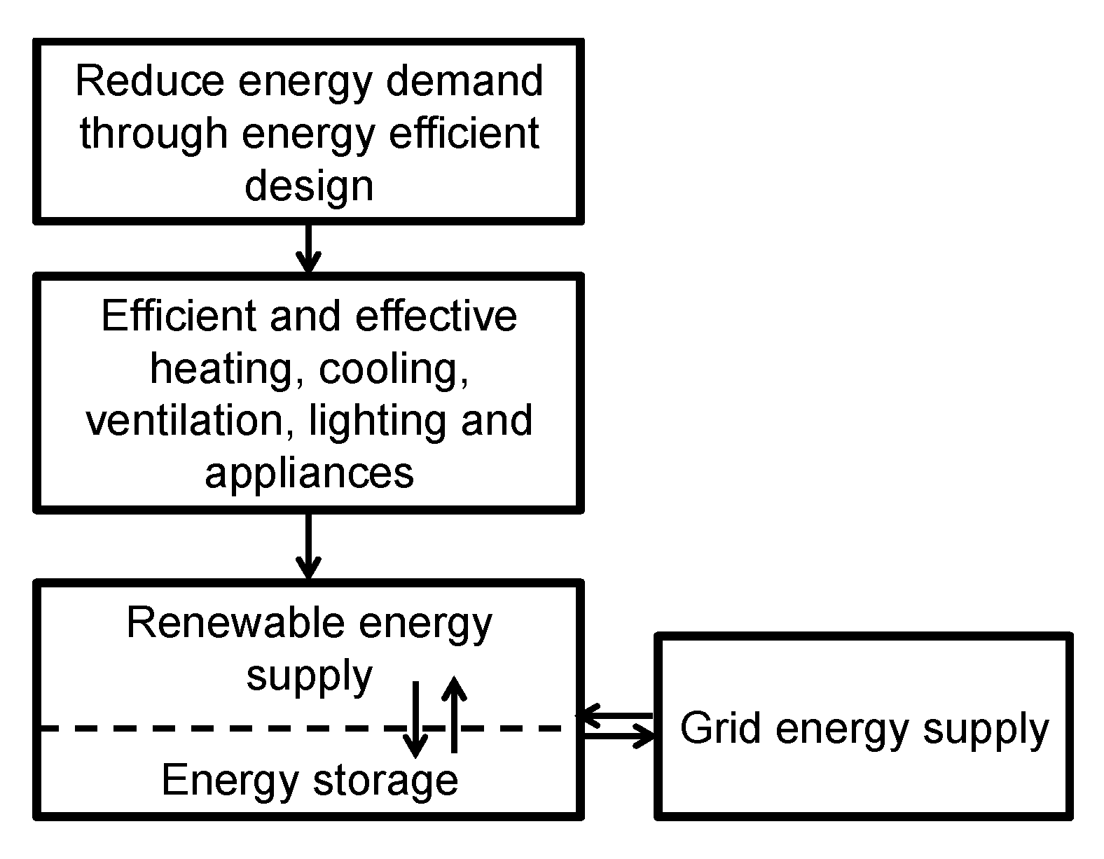
A systems approach, integrating reduced energy demand, renewable energy supply and energy storage has been shown to have the potential to deliver an energy-positive house performance (Figure 16). The integration of thermal and electrical technologies with architectural design features can potentially reduce costs and provide an improved aesthetic, in comparison to a more traditional ‘bolt-on’ technology approach which generally incurs a higher overall cost. The affordable construction costs make the house applicable for the housing market, especially for social housing, where low energy costs have greatest impact on householders.

The research has illustrated how a combination of energy modelling and detailed monitoring has led to a better understanding of how an energy-positive house performs and the relative contribution of its individual components combined within a whole systems approach. The analysis identified a performance gap, which was mainly attributed to infiltration between the heated space and roof space, disturbed thermal insulation in the ceiling and mechanical ventilation inlet and extract flows varying from their design specification. The performance gap identified would detract from the overall energy-positive performance, and potentially increase the annual heating costs by an estimated £140. This emphasises the need to ensure that a building is constructed to a good standard and that checks are made to identify any potential problems. This is especially the case with energy-positive performance where the energy demand is low and any performance gap can have a relatively higher impact on overall performance and the ability of systems to cope, in relation to their capacity to heat. A thermographic survey can identify major causes of poor thermal design and workmanship.

The study has indicated that, without a performance gap and with an efficient pattern of occupant use, the total electricity demand was predicted to be 4191 kWh/year (around 42 kWh/m²/year) with an annual grid import of 1112 kWh compared to the exported value of 1458 kWh. The building is predicted to import about 26% of its energy needs from the grid, but over the year its energy export to import ratio is 1.3:1. The annual space heating demand is 1464 kWh (14.64 kWh/m²), which is less than the 15 kWh/m² Passivhaus target. The results indicate that the space heating and DHW heating accounts for some 44% (1852 kWh/year) of the total electricity demand, with the remaining 66% (2339 kWh/year) used for other electrical demand (i.e., lights and appliances). The DHW heat demand is higher than that for space heating. The energy-positive performance can be further improved using water-efficient equipment, producing an annual energy export to import ratio rise to 1.4:1.

The performance of the MVHR and TSC contributes an equivalent of some 75% to the space heating, while the MVHR on its own contributes some 72% to space heating. The TSC is therefore of marginal benefit. However, it is potentially a relatively low-cost item and also provides the external element to the construction. A future modification to the house would be to use the TSC for all-year-round DHW heating, and possibly as a source for inter-seasonal chemical heat storage.

The results show the potential for energy-positive performance with existing technology and for an affordable cost, provided the performance gaps can be addressed. The SOLCER house has provided a detailed understanding of energy-positive performance, which is being followed up by the Welsh Government’s Innovative Housing Programme on a number of new social housing schemes [52].

References

- HM Government. Climate Change Act 2008 (c.27); Her Majesty’s Stationary Office Ltd.: London, UK, 2008; p. 1.
- BEIS. 2017 UK Green House Gas Emission, Provisional Figures; BEIS: London, UK, 2018.
- EPBD. Directive 2010/31/EU of the European Parliament and of the Council of 19 May 2010 on the Energy Performance of Buildings. Off. J. Eur. Union 2010, 53, 13–35. [Google Scholar]
- Stene, J.; Alonso, M.J.; Rønneseth, Ø.; Georges, L. State-of-the-Art Analysis of Nearly Zero Energy Buildings: Country Report IEA HPT Annex 49 Task 1-NORWAY; SINTEF Academic Press: Oslo, Norway, 2018. [Google Scholar]
- D’Agostino, D. Assessment of the progress towards the establishment of definitions of nearly zero energy buildings (nZEBs) in European member states. J. Build. Eng. 2015, 1, 20–32. [Google Scholar] [CrossRef]
- Cao, X.; Dai, X.; Liu, J. Building energy-consumption status worldwide and the state-of-the-art technologies for zero-energy buildings during the past decade. Energy Build. 2016, 128, 198–213. [Google Scholar] [CrossRef]
- Chang, H.; Liu, Y.; Shen, J.; Xiang, C.; He, S.; Wan, Z.; Jiang, M.; Duan, C.; Shu, S. Experimental study on comprehensive utilization of solar energy and energy balance in an integrated solar house. Energy Convers. Manag. 2015, 105, 967–976. [Google Scholar] [CrossRef]
- Rubeis, T.; Nardi, I.; Ambrosini, D.; Paoletti, D. Is a self-sufficient building energy efficient? Lesson learned from a case study in Mediterranean climate. Appl. Energy 2018, 218, 131–145. [Google Scholar] [CrossRef]
- Kristiansen, A.B.; Ma, T.; Wang, R.Z. Perspectives on industrialized transportable solar powered zero energy buildings. Renew. Sustain. Energy Rev. 2019, 108, 112–124. [Google Scholar] [CrossRef]
- IEA. World Energy Outlook 2013: Executive Summary. November 2018. Available online: https://webstore.iea.org/download/summary/190?fileName=English-WEO-2018-ES.pdf (accessed on 7 March 2020).
- Ala-Juusela, M.; Crosbie, T.; Hukkalainen, M. Defining and operationalising the concept of en energy positive neighbourhood. Energy Convers. Manag. 2016, 125, 133–140. [Google Scholar] [CrossRef] [Green Version]
- Rodriguez-Ubinas, E.; Montero, C.; Porteros, M.; Vega, S.; Navarro, I.; Castillo-Cagigal, M.; Matallanas, E.; Gutiérrezc, A. Passive design strategies and performance of net energy plus houses. Energy Build. 2014, 83, 10–22. [Google Scholar] [CrossRef] [Green Version]
- Takase, K.; Kawashima, N.; Sato, K.; Ohnuma, Y. Practice of net positive energy house in the suburb of Tokyo. Energy Procedia 2017, 143, 112–118. [Google Scholar] [CrossRef]
- Bojić, M.; Nikolić, N.; Nikolić, D.; Skerlić, J.; Miletić, I. Toward a positive-net-energy residential building in Serbian conditions. Appl. Energy 2011, 88, 2407–2419. [Google Scholar] [CrossRef]
- Heinze, M.; Voss, K. Goal: Zero energy building exemplary experience based on the solar estate Solarsiedlung Freiburg am Schlierberg, Germany. J. Green Build. 2009, 4, 93–100. [Google Scholar] [CrossRef] [Green Version]
- Ascione, F.; Bianco, N.; Böttcher, O.; Kaltenbrunner, R.; Vanoli, G.P. Net zero-energy buildings in Germany: Design, model calibration and lessons learned from a case-study in Berlin. Energy Build. 2018, 133, 688–710. [Google Scholar] [CrossRef]
- Jin, Y.; Wang, L.; Xiong, Y.; Cai, H.; Li, Y.H.; Zhang, W.J. Feasibility studies on net zero energy building for climate considering: A case of “All Green House” for Datong, Shanxi, China. Energy Build. 2014, 85, 155–164. [Google Scholar] [CrossRef]
- Karlessi, T.; Kampelis, N.; Kolokotsa, D.; Santamouris, M.; Standardi, L.; Isidori, D.; Cristallic, C. The concept of smart and NZEB buildings and the integrated design approach. Procedia Eng. 2017, 180, 1316–1325. [Google Scholar] [CrossRef]
- Wu, W.; Skye, H.M.; Domanski, P.A. Selecting HVAC systems to achieve comfortable and cost-effective residential net-zero energy building. Appl. Energy 2018, 212, 577–591. [Google Scholar] [CrossRef]
- Wu, W.; Skye, H.M. Net-zero nation: HVAC and PV systems for residential net-zero energy buildings across the United States. Energy Convers. Manag. 2018, 177, 605–628. [Google Scholar] [CrossRef]
- Li, B.; Wild, P.; Rowe, A. Performance of a heat recovery ventilator coupled with an air-to-air heat pump for residential suites in Canadian cities. J. Build. Eng. 2019, 21, 343–354. [Google Scholar] [CrossRef]
- Slonski, M.; Schrag, T. Linear optimisation of a settlement towards energy-plus house standard. Energies 2019, 12, 210. [Google Scholar] [CrossRef] [Green Version]
- Facci, A.L.; Krastev, V.K.; Falcucci, G.; Ubertini, S. Smart integration of photovoltaic production, heat pump and thermal energy storage in residential application. Sol. Energy 2019, 192, 133–143. [Google Scholar] [CrossRef]
- Committee on Climate Change. UK Housing: Fit for the Future? Committee on Climate Change: London, UK, 2019. [Google Scholar]
- Keiner, D.; Ram, M.; Barbosa, L.D.S.N.S.; Bogdanov, D.; Breyer, C. Cost optimal self-consumption of PV prosumers with stationary batteries, heat pumps, thermal energy storage and electric vehicles across the world up to 2050. Sol. Energy 2019, 185, 406–423. [Google Scholar] [CrossRef]
- O’Shaughnessy, E.; Cutler, D.; Ardani, K.; Margolis, R. Solar plus: Optimization of distributed solar PV through battery storage and dispatchable load in residential buildings. Appl. Energy 2018, 213, 11–21. [Google Scholar] [CrossRef]
- Parra, D.; Walker, G.S.; Gillott, M. Are batteries the optimum PV-coupled energy storage for dwellings? Techno-economic comparison with hot water tanks in the UK. Energy Build. 2016, 116, 614–621. [Google Scholar] [CrossRef]
- Weniger, J.; Tjaden, T.; Quaschning, V. Sizing of residential PV battery systems. Energy Procedia 2014, 46, 78–87. [Google Scholar] [CrossRef] [Green Version]
- Tumminia, G.; Guarino, F.; Longo, S.; Ferraro, M.; Cellura, M.; Antonucci, V. Life cycle energy performances and environmental impacts of a prefabricated building module. Renew. Sustain. Energy Rev. 2018, 92, 272–283. [Google Scholar] [CrossRef]
- BEIS. Industrial Strategy: Construction Sector Deal. Available online: https://assets.publishing.service.gov.uk/government/uploads/system/uploads/attachment_data/file/731871/construction-sector-deal-print-single.pdf (accessed on 25 February 2020).
- Kampelis, N.; Gobakis, K.; Vagias, V.; Kolokotsa, D.; Standardi, L.; Isidori, D.; Cristalli, C.; Montagnino, F.M.; Paredes, F.; Muratore, P.; et al. Evaluation of the performance gap in industrial, residential & tertiary near-zero energy buildings. Energy Build. 2017, 148, 58–73. [Google Scholar]
- Belussi, L.; Barozzi, B.; Bellazzi, A.; Danza, L.; Devitofrancesco, A.; Fanciulli, C.; Ghellere, M.; Guazzi, G.; Meroni, I.; Salamone, F.; et al. A review of performance of zero energy buildiCngs and energy efficiency solutions. J. Build. Eng. 2019, 25, 100772. [Google Scholar] [CrossRef]
- Li, H.X.; Gül, M.; Yu, H.; Awad, H.; Al-Hussein, M. An energy performance monitoring, analysis and modelling framework for netzero energy homes (NZEHs). Energy Build. 2016, 126, 353–364. [Google Scholar] [CrossRef]
- De Wilde, P. The gap between predicted and measured energy performance of buildings: A framework for investigation. Autom. Constr. 2014, 41, 40–49. [Google Scholar] [CrossRef]
- Menezes, A.C.; Cripps, A.; Bouchlaghem, D.; Buswell, R. Predicted vs. actual energy performance of non-domestic buildings: Using post-occupancy evaluation data to reduce the performance gap. Appl. Energy 2012, 97, 355–364. [Google Scholar] [CrossRef] [Green Version]
- Was, K.; Radon, J.; Sadlowska-Salega, A. Maintenance of passive house standard in thel of long-term study on energy use in a prefabricated lightweigth passive house in Central Europe. Energies 2020, 13, 2801. [Google Scholar] [CrossRef]
- Magrini, A.; Lentini, G.; Cuman, S.; Bodrato, A.; Mareno, L. From neally zero energy buildings (NZEB) to positive energy buildings (PEB): The next challeng—The most recent European trenads with some notes on the energy analusis of a forerunner PEB example. Dev. Built Environ. 2020, 3, 100019. [Google Scholar] [CrossRef]
- Jones, P.; Irvine, S.; Guwy, A.; Masters, I.; Bowen, P. LCRI 2015: Overview of LCRI Research 2008 to 2015; LCRI Cardiff University: Cardiff, UK, 2015; ISBN 978-1-899895-18-2. [Google Scholar]
- Feist, W.; Schnieders, J.; Dorer, V.; Haas, A. Re-inventing air heating: Convenient and comfortable within the frame of the Passive House concept. Energy Build. 2005, 37, 1186–1203. [Google Scholar] [CrossRef]
- Welsh Government. The Building Regulations 2010, Conservation of Fuel and Power: Approved Document Part L -2014 L1A-New Dwelling. Available online: http://gov.wales/docs/desh/publications/160614building-regs-approved-document-l1a-new-dwellings-en.pdf (accessed on 25 October 2019).
- Coma Bassas, E.; Jones, P.J. Buildings as power stations’: An energy simulation tool for housing. Procedia Eng. 2015, 118, 58–71. [Google Scholar] [CrossRef] [Green Version]
- Lewis, P.T.; Alexander, D.K. HTB2: A flexible model for dynamic building simulation. Built Environ. 1990, 25, 7–16. [Google Scholar] [CrossRef]
- Oscar Faber and Partners. IEA Annex 1, Computer Modelling of Building Performance: Analyses of Avonbank Simulation; IEA: St. Albans, UK, 1980. [Google Scholar]
- Lomas, K.J.; Eppel, H.; Martin, C.J.; Bloomfield, D.P. Empirical validation of building energy simulation programs. Energy Build. 1997, 26, 253–275. [Google Scholar] [CrossRef]
- Neymark, J.; Judkoff, R.; Alexander, D.; Felsmann, C. IEA BESTEST Multi-Zone Non-Airflow In-Depth Diagnostic Cases. In Proceedings of the Building Simulation 2011 Conference, Sydney, NSW, Australia, 14–16 November 2011. [Google Scholar]
- Li, S.; Karava, P.; Savory, E.; Lin, W.E. Airflow and thermal analysis of flat and corrugated unglazed transpired solar collectors. Sol. Energy 2013, 91, 297–315. [Google Scholar] [CrossRef]
- CIBSE. CIBSE Guide C: Reference Data; The Chartered Institution of Building Services Engineers: London, UK, 2007. [Google Scholar]
- Zimmermann, J.; Evans, M.; Griggs, J.; King, N.; Harding, L. Household Electricity Survey: A Study of Domestic Electrical Product Usage; Intertek: Milton Keynes, UK, 2012. [Google Scholar]
- Energy Monitoring Company; Energy Saving Trust. Measurement of Domestic Hot Water Consumption in Dwellings; Energy Saving Trust: London, UK, 2008. [Google Scholar]
- BRE. The Government’s Standard Assessment Procedure for Energy Rating of Dwellings, 2012th ed.; BRE: Watford, UK, 2014. [Google Scholar]
- Perisoglou, E.; Patterson, J.; Stevenson, V.; Jenkins, H. Investigating the application of small scale transpired solar collectors as air preheaters for residential buildings. In Proceedings of the International Conference on Sustainability in Energy and Buildings, Chania, Greece, 5–7 July 2017. [Google Scholar]
- Welsh Government. £43 Million Investment in Housing for the Future. Available online: https://gov.wales/ps43-million-investment-housing-future (accessed on 28 October 2019).
Figure 1.
Concept for achieving net zero-energy and energy-positive (plus-energy) buildings [16].
Figure 2.
View of the south-facing elevation of the smart operation for a low carbon energy region (SOLCER) house and roof integrated solar PV array, with floor plans (600 mm grid).
Figure 3.
SOLCER house schematic of electrical and thermal system.
Figure 4.
Schematic diagram for simulating the integrated system approach for the SOLCER energy-positive house.
Figure 5.
(a) Schematic of the TSC submodel; (b) Temperature rise between the external air temperature and the TSC outflow, against solar radiation incident on the TSC panel. Measured data is from October 2015 to March 2016 (grey markers and trend line); predicted data (dotted black trend line).
Figure 6.
Measured (black) and predicted (red) air temperature rise through the MVHR versus the temperature difference between the inlet air and outlet air before the MVHR (October 2015 to March 2016).
Figure 7.
Hourly distribution of temperature rise through the TSC and MVHR (October 2015 to March 2016), comparing predicted (red) with measured (black) data.
Figure 8.
Electricity generation by PV vs. Solar on the PV panel (October 2015 to March 2016), comparing measured (grey markers and black trend line) and predicted (red line) data.
Figure 9.
(a) The air leakage through the loft hatch during a blower door pressure test. (b) Roof space floor (left) and a thermal image of the floor in the roof space (right), indicating increased heat loss shown by relatively warmer areas where the thermal insulation was disturbed.
Figure 10.
Comparison of measurements and predictions for the period 20–26 December 2015 (a) measured and (b) predicted. The diagram below the plots identifies the main measurement locations in the top graph.
Figure 11.
Weekday and weekend energy and water use profiles constructed from measured daily totals [48,49].
Figure 12.
(a,b). Winter sunny week: 29 January–4 February.
Figure 13.
(a,b) Summer sunny week: 16 July–22 July.
Figure 14.
Summary of annual energy demand and supply. The total solar PV power includes the power used by the house, the surplus PV power and the losses.
Figure 15.
Summary of monthly energy values.
Figure 16.
A systems approach to energy-positive design.