
Abstract
Objective. In proton therapy there is a need for proton optimised tissue-equivalent materials as existing phantom materials can produce large uncertainties in the determination of absorbed dose and range measurements. The aim of this work is to develop and characterise optimised tissue-equivalent materials for proton therapy. Approach. A mathematical model was developed to enable the formulation of epoxy-resin based tissue-equivalent materials that are optimised for all relevant interactions of protons with matter, as well as photon interactions, which play a role in the acquisition of CT numbers. This model developed formulations for vertebra bone- and skeletal muscle-equivalent plastic materials. The tissue equivalence of these new materials and commercial bone- and muscle-equivalent plastic materials were theoretical compared against biological tissue compositions. The new materials were manufactured and characterised by their mass density, relative stopping power (RSP) measurements, and CT scans to evaluate their tissue-equivalence. Main results. Results showed that existing tissue-equivalent materials can produce large uncertainties in proton therapy dosimetry. In particular commercial bone materials showed to have a relative difference up to 8% for range. On the contrary, the best optimised formulations were shown to mimic their target human tissues within 1%–2% for the mass density and RSP. Furthermore, their CT-predicted RSP agreed within 1%–2% of the experimental RSP, confirming their suitability as clinical phantom materials. Significance. We have developed a tool for the formulation of tissue-equivalent materials optimised for proton dosimetry. Our model has enabled the development of proton optimised tissue-equivalent materials which perform better than existing tissue-equivalent materials. These new materials will enable the advancement of clinical proton phantoms for accurate proton dosimetry.
Export citation and abstract BibTeX RIS

Original content from this work may be used under the terms of the Creative Commons Attribution 4.0 licence. Any further distribution of this work must maintain attribution to the author(s) and the title of the work, journal citation and DOI.
1. Introduction
Tissue-equivalent phantoms are a vital tool for planning and dosimetric verification in end-to-end radiotherapy audits (Clark et al 2015, Thomas et al 2017, Carlino et al 2018, Taylor et al 2022). Phantoms are typically defined as a body of material that interacts with a type of radiation in the same manner as a patient (ICRU 1993). Over the past 50 years, a variety of phantoms have been developed for radiation modalities such as x-ray and electron treatments (Stacey et al 1961, Griffith et al 1976, White et al 1977, White 1978). In recent years, the number of proton therapy centres within the UK and worldwide has vastly increased (Crellin 2018). As a consequence, several studies (Palmans et al 2002, Al-Sulaiti et al 2012, Grant et al 2014, Lourenço et al 2017) have been investigating the performance of existing phantom materials in proton beams. However, due to differences in radiation interaction with matter between photon and proton beams (Andreo et al 2017, Paganetti 2017), phantom materials previously used for x-ray phantoms (White 1974) are not optimised, or sometimes unsuitable, for proton therapy.
Current phantom materials have been developed to mimic electron density and Hounsfield Unit (HU) for imaging and x-ray treatments (White 1974). However, for suitable phantom materials aimed at proton therapy, HU, relative stopping power (RSP), relative scattering power and nuclear interaction quantities should be mimicked as closely as possible. For reference dosimetry, which is recommended to be performed in water, the IAEA TRS-398 (Andreo et al 2000) states that plastic phantom materials should not be used due to the lack of information regarding water to plastic fluence corrections. Uncertainties caused by the tissue-equivalence of phantom materials have been also highlighted by Farr et al (2021) for the commissioning of intensity-modulated proton therapy system. Proton phantom development work by the Imaging and Radiation Oncology Core (IROC) group (Grant et al 2014, Branco et al 2017, Lewis et al 2018) emphasises the importance of a careful selection in phantom materials to ensure the phantom is adapted for proton dosimetry. Grant et al (2014) showed the need for phantom materials that are optimised for proton therapy, as only 50% of materials selected passed the 5% uncertainty criteria for correctly assigning stopping powers. In particular, bone materials were shown to produce large uncertainties for proton measurements. Goma et al (2018) showed that bone-equivalent materials, used in the stoichiometric calibration process, could result in an additional 3.5% uncertainty in RSP which could also be considered as additional range uncertainty. This is emphasised in the work by Lewis et al (2018) which showed that certain commercial bone-equivalent materials could cause up to 35% error in proton range.
Historically, most phantom material studies were reported by White (1974) and Constantinou (1978), who developed solid and gel-based tissue-equivalent materials for x-ray, electron beams and particle therapy (neutrons and protons). For proton therapy dedicated substitute materials, only mass density and mass stopping power were used within their model (Constantinou 1978). The new formulations were tested in a collimated scattered proton beam and the proton range as well as lateral profiles of the formulated materials compared to real tissue samples. Since then, most development of tissue-equivalent material has become a commercial activity. However, many tissue-equivalent materials are still based on the work of White (White 1974, Leeds Test Objects 2014). Water-equivalent materials for proton dosimetry were explored by Lourenço et al (2017) who assessed the particle fluence in commercial plastics against new plastic formulations. Their work highlighted a possible avenue of improvement of current tissue-equivalent materials for proton therapy by formulating new water-equivalent plastics which matched water within 1% for low- and high-energy proton beams in terms of particle fluence. These materials were lately implemented into a proton range phantom and results showed the materials are not tissue-equivalent for range calculations within clinical treatment planning systems (TPS) (Cook et al 2022).
The aim of this work is to develop end-to-end audit phantom materials to be used to mimic the patient workflow from patient data acquisition and treatment planning to dose verification. For the phantom material to be used through the workflow of a patient undergoing proton therapy, the materials need to be tissue-equivalent for both imaging photon energies as well as therapeutic proton energies to ensure the material is correctly characterised and provides accurate dosimetry of the target tissue. To our knowledge, this is the first model that enables the formulation of tissue-equivalent materials which considers not only photon interactions but also proton stopping power, nuclear absorption, and scattering interactions. The tissue-equivalence of the optimised materials were also compared against existing commercial tissue-equivalent materials to evaluate the performance of the latter and the improvement achieved with the new materials. Through the use of this model, new epoxy-resin based bone and muscle materials were made at the Barts Health NHS Trust using the manufacture process based on the work by White (1977). These manufactured materials were characterised by Monte Carlo simulations and experimental testing to assess their suitability for clinical use.
2. Methods
2.1. Epoxy-resin-based manufacture
In this study, the tissue-equivalent materials developed were based on epoxy-resin base mixtures (White et al 1977, Constantinou 1978, White 1974, 1977, 1978). The manufacture of epoxy resin-based tissue substitutes has been well described by White (1977). In summary, for the development of tissue-substitute materials, an epoxy resin, hardener, and selected powders or liquids are mixed to achieve a formulation with the required radiation properties of a desired target tissue. For successful hardening of the tissue-equivalent material, a specific mix ratio of epoxy resin and hardener is required; the different epoxy resin and hardener ratios are defined by White (1974) and were given the names CB1, CB2, CB3 and CB4. In this work, CB4 was used as that combination has been thoroughly tested (White 1974) and can be used to produce larger cast volumes required for phantom development (White 1977). Typically, the mass density of epoxy resins are greater than that of soft tissue (Xu and Eckerman 2009), hence low density microspheres, such as phenolic microspheres, are typically added to the mixture to achieve the required mass density of the material without significant change to the elemental formulation (White 1977). The mixture is vacuumed during and/or after mixing to remove any possible air bubbles and left to cure over a few days.
2.2. Mathematical model
The aim of the model was to find which material ratios produce adequate target tissue mimicking properties for photon imaging beams as well as therapeutic proton beams. A list of 89 components was created based on the work of White (1974) and Constantinou (1978). The selected components were affordable (<£2 per gram) and non-hazardous. To create a material, CB4 was mixed with phenolic microspheres and N additional components. The mass ratios in which the epoxy, phenolic microspheres, and components are mixed dictate the final radiation properties of the mixture.
2.2.1. Mass density
The mass density of the material,  needs to be mimicked to ensure that beam characteristics such as photon attenuation and proton range are the same as the target tissue. The conservation of volumes for material mixtures was assumed, which implies that no air is added into the mixture, that solid powders dissolve into the liquid without reducing the total volume and that chemical reactions also do not alter the volume. This results in the following formulation for the material's mass density:

The index  represents one of the
  mixture materials, and
  are respectively the mass fractional weight and mass density of the material constituents of the mixture.
2.2.2. Mass attenuation coefficient
For photon interactions, the photon mass attenuation coefficient of the material,  is the main beam interaction that needs to be considered for CT imaging (Andreo et al
2017). For mixtures, it is obtained as
is the main beam interaction that needs to be considered for CT imaging (Andreo et al
2017). For mixtures, it is obtained as

where  is the energy-dependent mass attenuation coefficient of the
  material in the mixture, and
  is the normalised spectrum of the polyenergetic x-ray source used for imaging. A 100 kVp clinical spectrum was used in the model.
2.2.3. Hounsfield unit
Multiplying  with the density provides the linear attenuation coefficient of the material,
  which can be used to calculate the HU of the material:

where,  is the linear attenuation coefficient of water. The HU is the quantity used to calculate the respective RSP of the material via the stoichiometric calibration curve (Schneider et al
1996).
is the linear attenuation coefficient of water. The HU is the quantity used to calculate the respective RSP of the material via the stoichiometric calibration curve (Schneider et al
1996).
2.2.4. Relative stopping power
The electronic stopping power  is calculated via the Bethe equation assuming that other terms in the stopping power expression do not play a significant role in the clinical proton energy range

where  is the electron radius,
  is the electron rest mass,
  the speed of light,
  is the atomic mass unit, and
  is the proton velocity in units of the velocity of light.
  of the material was calculated using the rule of mixtures, where
  and
and  respectively represent the atomic number and atomic mass of the mixture.
  is the mean excitation energy of the mixture in the condensed phase calculated using the Bragg additivity rule (ICRU 1993):

The mass electronic stopping power was determined over the energy range 50–250 MeV and then averaged. The average RSP of the mixed material,  is calculated as the ratio of the electronic stopping power of the material to that of water:

2.2.5. Nuclear interactions
Firstly, the nuclear reaction cross-section was calculated as it represents the probability of a primary proton being removed from the beam by a nuclear interaction. The linear energy transferred to secondary protons and alpha particles was also calculated at low and high proton beam energies ( = 50 and
  = 200 MeV). Secondary proton and alpha particles were chosen because those are the secondary particles that contribute most significantly to dose in low-Z materials (Lourenço et al
2016). Cross-section data from ICRU Report 63 were used (ICRU 2000).
= 200 MeV). Secondary proton and alpha particles were chosen because those are the secondary particles that contribute most significantly to dose in low-Z materials (Lourenço et al
2016). Cross-section data from ICRU Report 63 were used (ICRU 2000).
The nuclear reaction cross section of the mixture at energy  per atomic mass,
  in units of cm2 g−1, was calculated with the rule of mixtures (ICRU 2000):

The linear energy transferred from a proton of energy  to a secondary particle
  where
where  is a proton or an alpha particle, is defined as
  with units of MeV cm2 g−1, is calculated using:

where  is the average emission energy of the recoil spectrum.
The sum of the nuclear interactions cross sections value was calculated to give them equal weighting in the cost function:

2.2.6. Scattering length
The elemental scattering length,  was estimated as (Gottschalk 2010):

where  is the fine structure constant and
  is Avogadro's constant. The scattering length of mixtures is obtained with equation (11):

2.2.7. Cost function
A cost function was established to quantify the similarity between a mixture and a target material. The cost function is a weighted sum of the square of relative differences between 6 properties of the target and mixture material. The 6 quantities (noted with index  ) are the mass density
  (equation (1)), mass attenuation coefficient
  (equation (2)), HUm
(equation (3)), relative stopping power
(equation (2)), HUm
(equation (3)), relative stopping power  (equation (6)), scattering length
  (equation (10)) and sum of nuclear interaction cross sections (equation (9)). Ultimately, all properties depend upon the mass fractional weights
  of the
  components of the mixture, which are the optimisation variables. The cost function is defined as

where  is the relative difference on the
  quantity between target material and the proposed mixture, and
  is an empirically defined weighting of the relative importance of each quantity (see table 1). Mass density, mass attenuation and RSP were assigned higher weights due to their impact on the materials ability to be correctly characterised during imaging and TPS planning as well as providing accurate proton dosimetry and range measurements.
Table 1. Description of material formulation input settings and cost function weighting,  used for each formulation. For VB#1 and MS#H, the compound library was limited to only components used in current manufacture of photon tissue-equivalent materials at Barts Health NHS Trust (White 1974) or had been shown to mix well during the study. For the other iterations, VB#2, MS#1–3 the full component library was considered minus the powder previously used in earlier formulations.
| Cost function weightings | ||||||||||
|---|---|---|---|---|---|---|---|---|---|---|
| Name of material formulation | Target tissue | Component library (N) | Component properties | N | Density | Spectrum weighted mass attenuation | RSP | Scattering length | Average nuclear interaction | HU |
| VB#1 | Vertebra Column (C4) (excluding cartilage) | 3 | Fine powders | 1 | 0.21 | 0.26 | 0.26 | 0.13 | 0.13 | 0 |
| VB#2 | 89 | Liquid and powders | 1 | 0.21 | 0.26 | 0.26 | 0.13 | 0.13 | 0 | |
| MS#1 | ICRP Skeletal Muscle 2 | 89 | Liquid and powders | 1 | 0.21 | 0.26 | 0.26 | 0.13 | 0.13 | 0 |
| MS#2 | 88 | Liquid and powder | 1 | 0.17 | 0.22 | 0.22 | 0.11 | 0.11 | 0.17 | |
| MS#3 | 87 | Liquid and powders | 1 | 0.17 | 0.22 | 0.22 | 0.11 | 0.11 | 0.17 | |
| MS#H | 4 | Fine powders | 2 | 0.5 | 0.5 | 0 | 0 | 0 | 0 | |
The optimisation of the new formulation was achieved by finding a local minimum of the cost function using a constrained nonlinear least squares algorithm. The model was implemented in Matlab R2020b (MathWorks, Natick, MA, U.S.A.). The function was constrained by two conditions mainly linked to the manufacturing process for epoxy resin-based materials:
- (i)A minimum of
 = 60% CB4 was set as the lower limit for the epoxy resin in the model. This ensures that the components would be mixable and pourable in the manufacturing stage.
 - (ii)Overall, the formulation was set either parameters to optimise (mass fractional weight of CB4, mass fractional weight of phenolic microspheres and mass fractional weight of one or two mixture component). The number of mixture components was set to either N = 1 or 2 component per mixture to reduce the complexity of the manufacture process. Phenolic microspheres were always considered in the mixture formulation to easily ensure matching the density of the targeted material.


The optimal material was selected as the one with the lowest cost function.
2.3. Implementation of the mathematical model
The main challenge was to formulate materials that could be successfully mixed and poured, and that resulted in a homogeneous final material. Although the model provides a fast method for the formulation of theoretical proton optimised tissue-equivalent materials, the manufacture process remained a trial-and-error method and multiple materials were developed during this study. This was mainly due to the selected component powders not being fine enough to ensure homogenous mixing into the CB4 mixture; crystalline powders were shown to sink during the curing process. Consequently, the number of components used from the library was constantly revised during the study as selected powders were shown to be unsuccessful in the mixing process.
The model was used to formulate a vertebra bone-equivalent (two samples were formulated, VB#1–2) and skeletal muscle-equivalent material (five samples formulated, MS#1, MS#2, MS#3, MS#3 v2 and MS#H) based on Woodard and White (Woodard and White 1986) and ICRP reference tissue data (Snyder et al
1975). Photon and proton interactions were also calculated for current commercial tissue-equivalent materials (CIRS Inc. (CIRS 2020), Leeds Test Object (Leeds Test Objects 2014), and Gammex Inc. (Sun Nuclear 2019) against selected human tissues. For commercial materials, the material density and elemental composition data was taken from published documentation (Leeds Test Objects 2014, Goma et al
2018). Table 1 shows the material formulation input settings and cost function weightings ( ) for each quantity
  considered in the model for each mixture.
For VB#1–2 and MS#1, the cost function weighting for HU was set to zero due the initial model only considering the spectrum weighted mass attenuation parameter. These first formulations highlighted the importance of accurately matching the HU quantity to ensure correct TPS RSP assignment. Consequently, for MS#2–3, a weighting value was used for HU in the cost function. Also, after the manufacture of MS#3, the formulation was adjusted by the addition of less than 1% of phenolic microspheres to alter the density to better mimic the target tissue density, this formulation was named MS#3 v2. During the study, the development of a homogenous muscle was shown to be challenging, due its importance in the photon imaging and TPS characterisation stage, a less optimised but more homogenous mixture was developed called MS#H.
2.4. Monte Carlo validation of the mixtures
Monte Carlo simulations were performed for validation of the theoretical radiation properties of the materials calculated via the mathematical model by simulating a proton beam travelling through a given thickness of human tissue and tissue-equivalent materials. Monte Carlo simulations were performed with FLUKA 2021.2.1 and Flair 2.3.0 (Vlachoudis 2009, Battistoni et al 2015, Ahdida et al 2022). The range, RSP, and fluence correction factor were evaluated with the Monte Carlo simulations, as defined in sections 2.4.1 and 2.4.2. For each simulation, 6 × 10⁶ proton histories were tracked and the beam was modelled as a mono-directional 200 MeV pencil beam. The default settings for particle therapy were used with full transport of ions (inelastic scattering, elastic scattering, and nuclear interactions) while secondary electrons were set to deposit dose locally. The transport cut-off energies for proton and heavier particles were set to 100 keV. The elemental composition, density, and theoretical calculated I-value of the materials were entered into the material information. For newly formulated materials, the mathematical model derived theoretical density was used. Existing commercial bone and muscle solutions were also assessed. All materials were modelled as homogeneous within the simulations. A cylindrical target of radius 30.0 cm and thickness of 26.0 cm was modelled, and the total dose was scored in 0.2 cm thick slabs throughout the target. The dose distribution and fluence for primary protons, secondary protons, alpha, He3, deuterons and tritons were scored throughout the cylinder.
2.4.1. Range and RSP
The percentage depth dose (PDD) for the proton beam in each material was calculated. The range was determined from the PDD and was defined as the  the depth distal to the Bragg peak where the PDD drops to 80%. The range also provides the RSP
  which is determined by the following equation:

where  is the distal
  range in water and
  is the distal
  range in the target material.
2.4.2. Fluence correction factor
The fluence correction factor,  provides information on the difference in fluence between materials (Palmans et al
2013, Lourenço et al
2016), and was calculated as described in Palmans et al (2013). The fluence difference provides an understanding of the differences in non-elastic nuclear cross sections of the material compared to the target tissue. Consequently, if
provides information on the difference in fluence between materials (Palmans et al
2013, Lourenço et al
2016), and was calculated as described in Palmans et al (2013). The fluence difference provides an understanding of the differences in non-elastic nuclear cross sections of the material compared to the target tissue. Consequently, if  this suggests that the material and target tissue are equivalent in terms of particle fluence (Palmans et al
2013).
this suggests that the material and target tissue are equivalent in terms of particle fluence (Palmans et al
2013).
2.5. Experimental validation of the mixtures
The formulations were manufactured by the Barts Health NHS Trust and a series of tests were performed at the National Physical Laboratory (NPL, UK), University College London Hospital Proton Centre (UCLHPC), and the Rutherford Cancer Centre Thames Valley (RCCTV) to characterise the materials to ensure they were within suitable uncertainties for use in proton therapy. For each formulation, three blocks were manufactured with the following dimensions: 10 cm×10 cm slabs of 0.5 cm, 1.0 cm and 2.0 cm thickness.
2.5.1. Density
The measured material density of the three individual slabs was calculated by weighing them on a Mettler Toledo analytical balance (Model PG503 S) and performing length measurements with Mitutoyo Absolute IP 67 digital callipers (Model CD 8PSX).
2.5.2. Relative Stopping Power
Measurements were taken at UCLHPC using a mono-energetic proton beam. The IBA Giraffe device (IBA Dosimetry) was used to provide a complete PDD curve in one irradiation. For VB#1–2 a 140 MeV proton beam was used. For MS#1–3 and MS#H, a 200 MeV proton beam was used. It should be noted that water-equivalent thickness measurements do not depend significantly on energy over the clinical proton energy range (Zhang and Newhauser 2009).
At both energies, a reference PDD was initially taken without an additional material (figure 1, setup 1). Then each slab of material was placed in front of the entrance window of the detector, and the PDD measurement repeated for each material (figure 1, setup 2). PDD measurements were performed to determine the water equivalent thickness  and RSP of the materials (
 ), using equations (14) and (15), respectively (Newhauser and Zhang 2015).


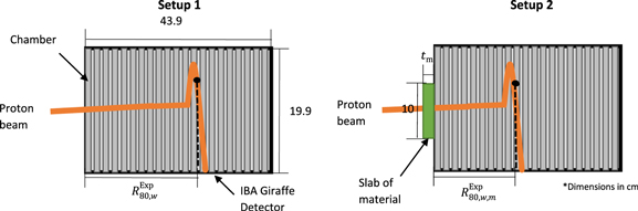
Figure 1. Experimental setup for water-equivalent thickness measurements (without - setup 1, left - and with - setup 2, right – phantom material in front of the Giraffe detector). The number of ionization chambers shown within detector is reduced to simplify the schematic.
Download figure:
Standard image High-resolution image
 corresponds to the range in water,
  is the
  range in water when including the material slab in front of the water phantom and
  the thickness of the material slab. The
  values were determined via the IBA detector software which applied the Bortfeld fit to the Bragg peak curve before interpolating the
  range (Bortfeld 1997). Thickness measurements of the slabs was determined by dimensional measurements (section 2.5.1).
2.5.3. Single-energy CT and Dual-energy CT
Each slab was scanned in a Mediso AnyScan SCP scanner at the NPL. The samples were placed centrally within custom made inset within bolus sheets and solid water was placed above and below the setup on the carbon fibre CT couch (figure 2). This custom made inset for the samples was developed to reduce scattering and artefacts in the scan due to air. The following scanner settings were used; axial scan, 80 kV, 100 kV, 120 kV and 140 kV tube voltages, voxel size of 0.098 × 0.098 × 0.125 cm3, tube current of 300 mA and scan reconstruction of abdomen. Each slab (0.5 cm, 1.0 cm, and 2.0 cm) was scanned separately as well as scanned together as a 10 cm×10 cm × 3.5 cm block.

Figure 2. Schematic of CT scanning phantom material setup.
Download figure:
Standard image High-resolution imageCT scans were also performed on two clinical CT scanners; the Philips CT 7500 scanner at the UCLHPC and the Philips Big Bore CT scanner at the RCCTV, using 120 kV tube voltage and similar setting as the scans aforementioned.
2.5.3.1. Homogeneity
Homogeneity of the samples was tested through visual assessment of the single-energy CT (SECT) images taken at NPL. Visual examination looked for any air bubbles and marbling effects in slices from the CT images as well as assessment of the materials variability through HU standard deviation (SD) calculations for each sample. The SD of the HU values of the samples was compared to WT1 to quantitively assess their homogeneity. WT1 is a commercial photon solid water equivalent material that has been shown to be acceptably homogeneous and it is extensively used in conventional radiotherapy. A plastic bottle filled with distilled water was also scanned alongside the samples to provide information on HU variation due to CT scanner noise.
2.5.3.2. HU and CT-based RSP estimation
Raystation 10B (version 10.1.100) was used to determine the HU of the material by manual contouring the central regions of each slab. The average HU values of the materials were derived from taking the HU value of the individual slabs (0.5 cm, 1.0 cm and 2.0 cm) as well as the combined 3.5 cm thick slab setup. The HU values for the three individual slab thicknesses were then applied to the stoichiometric calibration curves and the average predicted  and respective SD were determined for each scanner. At NPL, SECT and Dual-energy CT (DECT) analysis was completed to predict
  For DECT, the stoichiometric method of (Bourque et al
2014) was applied to the 100 kV and 140 kV scan data. The assigned
For DECT, the stoichiometric method of (Bourque et al
2014) was applied to the 100 kV and 140 kV scan data. The assigned  were then compared to experimentally derived
  values.
3. Results
3.1. Mathematical model calculations
Table 2(a) shows the relative difference of physical and radiation parameters between the new vertebra bone formulations and commercial bone materials against human vertebra bone. Similarly, table 2(b) shows the relative difference of physical and radiation parameters between the new skeletal muscle formulations and commercial muscle materials against the skeletal muscle. A cost function value of zero would suggest that all radiation parameters match to the target tissue.
Table 2. (a) Comparison of new formulations and commercial bone materials against vertebra bone, (b) comparison of new formulation and commercial muscle materials against skeletal muscle. For the cost function (1), the weightings shown in table 1 for formulations VB#1–2 and MS#1 were used and for cost function (2) the weighting shown in table 1 for MS#2–3 were used which included a HU weighting.
| Relative % difference to target tissue | VB#1 | VB#2 | CIRS Bone 800 mg/c.c. HA | Gammex Bone #480 | Gammex Bone #484 | Leeds test object (Average bone) | ||||
|---|---|---|---|---|---|---|---|---|---|---|
| a | ||||||||||
| Mass density | 1.41 | 0.70 | 7.75 | 9.86 | −5.99 | −1.41 | ||||
| Mass attenuation coefficient | 1.16 | 0.46 | 18.83 | 8.09 | −10.90 | −6.96 | ||||
| RSP | −0.12 | −0.67 | 6.63 | 8.20 | −4.02 | −0.85 | ||||
| Scattering length | 1.02 | 0.54 | −11.45 | −10.20 | 20.57 | 10.85 | ||||
| Average nuclear interactions | 2.61 | 1.65 | 1.82 | 1.57 | 5.42 | 4.47 | ||||
| Cost function (1) | 1.79 | 0.66 | 133.66 | 68.76 | 101.43 | 31.09 | ||||
| Relative % difference to target tissue | MS#1 | MS#2 | MS#3 | MS#H | CIRS Muscle | Gammex Muscle | ||||
| b | ||||||||||
| Mass density | 1.90 | 0.95 | 0.95 | 0.00 | 1.14 | 0.00 | ||||
| HU | 65.61 | 0.25 | −0.54 | 0.00 | 1.53 | −18.71 | ||||
| Mass attenuation coefficient | 1.00 | −0.93 | −0.97 | 0.00 | −1.06 | −0.83 | ||||
| RSP | −1.34 | −1.20 | −1.16 | −0.35 | 1.28 | −1.18 | ||||
| Scattering length | 0.62 | 7.60 | 7.67 | 10.87 | 11.24 | 10.51 | ||||
| Average nuclear interactions | 2.86 | 4.93 | 5.06 | 5.48 | 5.84 | 5.44 | ||||
| Cost function (1) | 2.61 | 11.46 | 11.76 | 19.29 | 21.86 | 18.75 | ||||
| Cost function (2) | N/A | 9.70 | 9.99 | 16.32 | 18.88 | 75.39 | ||||
3.2. Validation of material radiation parameters
3.2.1. Monte Carlo simulations
3.2.1.1. Range and RSP measurements
The relative difference between the mathematical model and Monte Carlo simulation predicted RSP was 0.4% (SD = 0.4%). Figure 3 shows  and
and  values determined from the simulation for the VB#1–2, MS#1–3 and MS#H, and commercial tissue-equivalent materials as well as their corresponding target tissues, vertebra bone, and skeletal muscle for a 200 MeV proton beam.
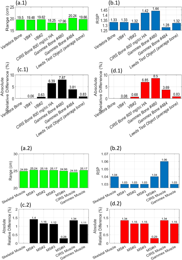
Figure 3. Monte Carlo derived  and
and  values of all new formulations (VB#1-2, MS#1-3 and MS#H) and commerical materials for a 200 MeV proton beam.
  values for vertebra bone and vertebra bone plastics are presented in figure 3(a.1) while
  values for muscle, and muscle plastics are presented in figure 3(a.2). Their respective relative difference to the target tissue are presented in figures 3(c.1) and (c.2).
  values for vertebra bone plastics are presented in figure 3(b.1) while
  values for muscle plastics are presented in figure 3(a.2). Their respective relative difference to the target tissue is presented in figures 3(d.1) and 3(d.2).
Download figure:
Standard image High-resolution image3.2.1.2. Fluence correction factors
Figure 4 shows the fluence correction factor of each newly formulated material and commercial materials for each target material. The depth was scaled to the range of the target tissue.

Figure 4. Fluence correction factors for new formulations and commercial materials. (a) Vertebra bone tissue-equivalent materials (b) muscle tissue-equivalent materials. Reference dashed lines highlighted maximum tissue thicknesses of each target tissue a proton may pass through in a patient (4 cm for bone and 15 cm for muscle). Type A uncertainties are presented with each error bar.
Download figure:
Standard image High-resolution image3.2.2. Measurements
3.2.2.1. Homogeneity
Table 3 and figure 5 shows the HU values and CT scans of each new formulation. Although no material showed air bubbles, heterogeneity of samples can be seen in the scans. For MS#1, the setting of the component powder within the sample is clearly visible in figure 5. A SD level of 5 HU was attributed to scanner noise through investigating HU variation for a reference water bottle placed alongside the material scans.
Table 3. HU values (max, min, average and SD).
| Material | Min HU | Mean HU | Max HU | SD |
|---|---|---|---|---|
| WT1 | −38 | 9.17 | 44 | 8 |
| VB#1 | 546 | 634 | 705 | 20 |
| VB#2 | 490 | 611 | 675 | 20 |
| MS#1 | −178 | 82 | 439 | 190 |
| MS#2 | −388 | 47 | 141 | 59 |
| MS#3 | −44 | 52 | 110 | 21 |
| MS#3 v2 | −116 | 26 | 86 | 24 |
| MS#H | 6 | 48 | 79 | 10 |

Figure 5. Example CT slices of new formulations.
Download figure:
Standard image High-resolution image3.2.2.2. Density and measurements

Table 4 shows the experimental calculated mass density and  values for the new formulations, as well as relative difference to model-predicted values and to target tissues values. The mathematical model on average predicted the experimental material density within 1.3% (SD = 0.8%) and RSP within 2.5% (SD = 0.9%) when MS#1 is excluded. MS#1 shows significant variation in density between measured slabs due to its heterogeneous nature (figure 4(c)). For the vertebra bone materials, the experimental values were on average within 2.0% (SD = 0.6%) for mass density and
  with target human vertebra bone formulation. For the muscle materials, the experimental values were on average within 1.7% (SD = 1.1%) for mass density and
  with target human skeletal muscle formulation. For MS#3 and MS#3 v2, the addition of phenolic microspheres reduced the percentage point difference to the target skeletal muscle by 1.7 for mass density and 2.4 for
Table 4. Mass density and RSP measurements of samples.
| Material | VB#1 | VB#2 | MS#1 | MS#2 | MS#3 | MS#3 v2 | MS#H |
|---|---|---|---|---|---|---|---|
| Average mass density (SD) | 1.458 (<0.01) | 1.443 (<0.01) | 1.091 (0.19) | 1.056 (0.04) | 1.080 (0.01) | 1.055 (0.02) | 1.054 (<0.01) |
| Average relative % difference to model prediction (SD) | 1.25 (0.24) | 0.91 (0.25) | 12.21 (8.97) | 2.67 (1.43) | 1.79 (0.98) | 1.04 (0.22) | 0.36 (0.11) |
| Average relative % difference to target tissue (SD) | 2.69 (0.25) | 1.62 (0.25) | 13.21 (8.95) | 2.37 (2.20) | 2.85 (1.03) | 1.11 (1.13) | 0.37 (0.11) |
Average  (SD) (SD) | 1.354 (<0.01) | 1.342 (<0.01) | 1.058 (0.16) | 1.052 (0.01) | 1.067 (0.01) | 1.051 (0.01) | 1.061 (<0.01) |
| Average relative % difference to model prediction (SD) | 2.43 (0.23) | 2.08 (0.06) | 10.91 (6.47) | 2.14 (1.28) | 4.34 (0.65) | 2.08 (0.45) | 2.21 (0.23) |
| Average relative % difference to target tissue (SD) | 2.37 (0.24) | 1.44 (0.06) | 10.66 (7.34) | 0.98 (1.33) | 3.33 (0.07) | 0.91 (0.48) | 1.90 (0.24) |
3.2.2.3. HU and CT-based RSP estimation
Table 5 compares predicted  (using the CT stoichiometric calibration) from NPL, UCLHPC, and RCCTV, against experimental
  values taken at UCLHPC (section 2.5.2.). The table shows that at NPL, for all materials the
  can be assigned on average within 1.4% (SD = 0.5%) difference to the experimental
  when using single-energy CT. This is reduced to, on average, within 1.3% (SD = 0.5%) if dual energy CT is used. At UCLHPC, for all materials the correct
  can be assigned on average within 2.3% (SD = 0.9%) difference to experimental
  and for the RCCTV all materials can be assigned the correct
  within 1.9% (SD = 1.3%) difference to experimental
Table 5. Stoichiometric calibration results for SECT, DECT, and clinical CT. Due to MS#1 not being suitable for clinical use due to powder settling within sample, the sample was not CT scanned at UCLHPC and RCCTV.
| Location and type of CT scan | Material | VB#1 | VB#2 | MS#2 | MS#3 | MS#3 v2 | MS#H |
|---|---|---|---|---|---|---|---|
| NPL (SECT 120 kVp) | Average HU (SD) | 633 (10) | 609 (9) | 50 (22) | 52 (5) | 26 (12) | 48 (1) |
Average  (SD) (SD) | 1.377 (0.01) | 1.364 (0.01) | 1.049 (0.02) | 1.054 (0.01) | 1.034 (0.01) | 1.051 (<0.01) | |
Average relative % difference to experimental  (SD) (SD) | 1.67 (0.61) | 1.62 (0.43) | 0.57 (0.61) | 2.04 (0.67) | 1.61 (0.66) | 0.96 (0.23) | |
| NPL (DECT (100 kVp and 140 kVp) | Average HU (SD) | 704 (7) and 581 (12) | 674 (4) and 558 (11) | 52 (22) and 49 (22) | 49 (5.4) and 53 (6) | 24 (12) and 29 (11) | 50 (1) and 46 (1) |
Average  (SD) (SD) | 1.355 (0.10) | 1.346 (0.04) | 1.049 (0.03) | 1.060 (0.01) | 1.035 (0.01) | 1.050 (<0.01) | |
Average relative % difference to experimental  (SD) (SD) | 0.64 (0.48) | 1.91 (1.61) | 0.94 (0.82) | 1.50 (0.71) | 1.57 (0.89) | 1.10 (0.23) | |
| UCLH Proton Centre DECT (120 kVp, dual-layer) | Average HU (SD) | 692 (6) | 662 (7) | 47 (23) | 41 (9) | 16 (10) | 46 (1) |
Average  (SD) (SD) | 1.331 (<0.01) | 1.318 (<0.01) | 1.036 (0.02) | 1.034 (0.01) | 1.020 (0.01) | 1.038 (<0.01) | |
Average relative % difference to experimental  (SD) (SD) | 1.70 (0.36) | 1.74 (0.29) | 1.46 (0.65) | 3.89 (0.59) | 3.00 (0.39) | 2.24 (0.23) | |
| Rutherford Cancer Centre, Thames Valley (SECT 120 kVp) | Average HU (SD) | 621 (11) | 596 (10) | 40 (22) | 37 (6) | 15 (9) | N/A |
Average  (SD) (SD) | 1.345 (0.01) | 1.330 (0.01) | 1.037 (0.02) | 1.036 (0.01) | 1.022 (0.01) | N/A | |
Average relative % difference to experimental  (SD) (SD) | 0.69 (0.55) | 0.88 (0.43) | 1.38 (0.60) | 3.77 (0.69) | 2.76 (0.32) | N/A |
4. Discussion
Table 2 and figure 3 highlight the overall potential of the new formulations to perform better than current commercial tissue-equivalent materials. Table 2 shows new formulations score well (close to zero) via the weighted cost function which indicates their feasibility for providing improved proton dosimetry. Results also suggest good agreement between the mathematical model and Monte Carlo simulations values, where for  were on average within 0.35%. Figure 3 indicates that all formulated materials match the target tissue ranges within 0.78% whereas commercial bone materials showed to have a relative difference up to 8% for range.
However, unlike the mathematical model predictions of improved nuclear interactions, Monte Carlo shows the fluence correction of the new formulations are comparable to commercial tissue-equivalent materials. Therefore, this suggests a higher weighting of the nuclear interaction parameters may be necessary or the current parameter does not fully capture the nuclear interactions of the targeted material. Some uncertainty can be attributed to the nuclear data used in the model compared to Monte Carlo simulations. The model uses ICRU Report 63 data which reports uncertainties of the order 5%–30% for cross sectional data; whilst for FLUKA, the PEANUT nuclear model was used which uses a blend of experiment data, data driven theoretical approaches, particle data group fits and phase shift analysis (Ferrari and Sala 1993). Work by Lourenço et al 2017 reported at least 2% differences in fluence correction factors depending on the Monte Carlo code. Previous research has also highlighted the challenge of quantifying the probability of non-elastic nuclear interactions due to hydrogen content of compounds (Rasouli et al 2016). Consequently, consideration should be made to adapt the model to improve the optimisation of nuclear interactions.
From table 2, VB#1–2, MS#1 were shown to provide the best optimisation of radiation parameters, however, manufacture challenges meant formulations did not result in suitable homogenous mixtures. Figure 5 highlights the unsuccessful mixing of MS#1 into a homogenous mixture due to the powdered material settling within the mixture whilst it hardens. MS#1–2 showed (table 3) significant variation in HU from the mean which suggests that these materials should not be used for clinical phantom use. Significant HU variation of the material is an undesirable material trait for certain applications such as phantoms for reference dosimetry and profile measurements. However, for the use in anthropomorphic phantom for end-to-end audits, minor HU variation could be useful as this would simulate human tissue heterogeneity. This could provide rigorous testing of the TPS and dose calculations during the patient workflow audit. Nevertheless, the challenge of inhomogeneous plastics is capturing HU variation which is clinically relevant and distinguished within the CT image.
After a review of muscle iterations and the available powders, the optimisation was simplified and focused on the manufacture of a homogeneous material, MS#H. The development of a homogenous material was at the cost of optimising the phantom material for proton interactions and resulted in a formulation with a smaller uncertainty on the assignment of 
Overall, results from table 4 (excluding MS#1) indicated that the model can predict mass density and radiation properties within the relative standard uncertainty of the method of calculation. The model predicted the RSP and mass density of the materials within 1.5% (when RSP calculations are corrected for experimental density values). Table 4 also shows for both the vertebra bone and muscle materials, that formulations were on average within 2% for mass density and  of the human target tissues. Results indicate VB#2 and MS#3 v2 are the most suitable bone and muscle-equivalent materials and outperform many of the existing materials. Major improvements were achieved in comparison to commercial bone materials, which showed relative differences up to 10% and 8% respectively for mass density and
  (table 2).
The materials were also assessed for their use as phantom materials for audit purposes. As previously mentioned, the acceptance criteria of phantom materials for IROC phantom development (Grant et al
2014) is a 5% uncertainty in TPS assigned RSP. Results from SECT and DECT scans at NPL and clinical centres (UCLHPC and RCCTV) suggest the materials  can be correctly assigned within 1%–3% (table 5). The improved homogeneity of MS#H also showed to improve the consistency and accuracy of
  assignment. Consequently, the optimised materials
  assignment is clearly within the 5% uncertainty IROC phantom material acceptance criteria and with certain phantom iterations the
  uncertainty is likely to be masked within the uncertainty of other steps in the phantom audit process such as setup and dosimeter measurement.
Future work will look to apply this model to manufacture proton optimised water and other human tissues (lung and denser bone) materials as well as be applied to support research into 3D printable based optimised materials.
5. Conclusion
The model developed is a powerful tool for the formulation of tissue-equivalent materials optimised for proton dosimetry. In previous research, Lewis et al (2018), existing bone materials have been shown to produce large uncertainties for range measurements. This work agrees with this finding as selected existing bone plastics have shown to produce up to 20% relative difference to the vertebra bone for key proton radiation parameters. This model enabled the creation of new proton optimised tissue-equivalent materials which are superior than current commercial bone and muscle materials when both mass density, photon interactions and proton interactions are determined via a weighted cost function.
Manufactured materials were characterised by Monte Carlo simulations and experimental testing and results suggest VB#2 and MS#3 v2 are the most tissue-equivalent (within 2% relative difference for key radiation parameters) and perform better than existing tissue-equivalent materials. The materials were also tested as audit materials by comparing stoichiometric calibration predicted and experimental determined RSP. Overall, for the new materials formulated, TPS predicted the experimental RSP values within 1%–3%, and consequently they can be used as clinical phantom materials. VB#2, MS#3 v2, and MS#H as well as future materials developed by the model will be used within clinical phantoms to improve phantom dosimetry measurements.
Acknowledgments
The authors would like to thank the medical physicists and proton beam engineers at University College London Hospital, Proton Centre and The Rutherford Cancer centre, Thames Valley for their assistance during the experiments. As well as the Barts Health NHS Trust staff for helping in the manufacture of the new phantom materials. This work was supported by the National Measurement System of the UK's Department for Business, Energy, and Industrial Strategy.